Lecture 7
Unsupervised Learning: Clustering and PCA
April 13, 2026
🗂🧭️ Clustering and Principal Component Analysis
🤖 Unsupervised Learning
- Unsupervised learning methods discover unknown relationships in data.
- With unsupervised methods, there’s no outcome that we’re trying to predict.
- Instead, we want to discover patterns in the data that perhaps we hadn’t previously suspected.
- Unsupervised learning: ML + Data Visualization
- Instead, we want to discover patterns in the data that perhaps we hadn’t previously suspected.
- We look at three classes of unsupervised methods:
- Cluster analysis finds groups with similar characteristics.
- Principal component analysis (PCA) turns many variables into a few new ones, called principal components, that still capture most of our data. (PCA is a popular dimensionality reduction method!)
- Association rule learning discovers relationships between variables — for example, which items tend to be purchased together.
🗂️ Clustering
- In cluster analysis, the goal is to group the observations in our data into clusters such that every observation in a cluster is more similar to other observations in the same cluster than observations in other clusters.
- E.g., a company that offers guided tours might want to cluster its clients by behavior and tastes:
- Which countries they like to visit
- Whether they prefer adventure tours, luxury tours, or educational tours
- What kinds of activities they participate in
- What sorts of sites they like to visit
- E.g., a company that offers guided tours might want to cluster its clients by behavior and tastes:
🥩 Protein Consumption Data
- To demonstrate clustering, we will use a small dataset from 1973 on protein consumption from 9 different food variables in 25 countries in Europe.
- The goal is to group the countries based on patterns in their protein consumption.
⚖️ Units and Scaling
- The units we choose to measure our data can significantly influence the clusters that an algorithm uncovers.
- One way to try to make the units of each variable more compatible is to standardize all the variables to have a mean value of 0 and a standard deviation of 1.
# Uses all columns except the first (Country)
vars_to_use <- colnames(protein)[-1]

# Scale to mean 0, sd 1; stores center and scale attributes
pmatrix <- scale(protein[, vars_to_use])
pcenter <- attr(pmatrix, "scaled:center")
pscale  <- attr(pmatrix, "scaled:scale")

# Convenience function to strip scale attributes
rm_scales <- function(scaled_matrix) {
  attr(scaled_matrix, "scaled:center") <- NULL
  attr(scaled_matrix, "scaled:scale")  <- NULL
  scaled_matrix
}

pmatrix <- rm_scales(pmatrix)- We can scale numeric data in R using the function
scale(). - The
scale()function annotates its output with two attributes:scaled:centerreturns the mean values of all the columns;scaled:scalereturns the standard deviations.
📊 Density Plots — Raw vs. Scaled
df_raw    <- protein |> select(FrVeg, RedMeat) |> mutate(type = "Original")
df_scaled <- as.data.frame(pmatrix) |>
               select(FrVeg, RedMeat) |>
               mutate(type = "Scaled")

bind_rows(df_raw, df_scaled) |>
  pivot_longer(c(FrVeg, RedMeat), names_to = "variable", values_to = "value") |>
  ggplot(aes(x = value, color = variable)) +
  geom_density(linewidth = 1) +
  facet_wrap(~type, scales = "free") +
  labs(title = "Raw vs. Scaled Distributions", color = NULL)
🌳 Hierarchical Clustering — Dendrogram
Hierarchical clustering builds a tree of nested groupings, called a dendrogram.
rownames(pmatrix) <- protein$Country
distmat <- dist(pmatrix, method = "euclidean")
pfit    <- hclust(distmat, method = "ward.D")

p <- fviz_dend(pfit, k = 5,
               rect        = TRUE,
               rect_fill   = TRUE,
               rect_border = "gray40",
               main        = "Ward Dendrogram — Protein Data",
               xlab        = "", ylab = "Height",
               cex         = 0.75) +
  theme(legend.position = "none")

# Thin the branch segments by overriding linewidth in every segment layer
for (i in seq_along(p$layers)) {
  if (inherits(p$layers[[i]]$geom, "GeomSegment")) {
    p$layers[[i]]$aes_params$linewidth <- 0.5
    p$layers[[i]]$aes_params$size      <- 0.5
  }
}
phclust()uses one of a variety of clustering methods to produce a tree that records the nested cluster structure.- Here we choose Ward’s method.
hclust()takes a distance matrix fromdist()as input.
📐 Ward’s Method and Within Sum of Squares (WSS)
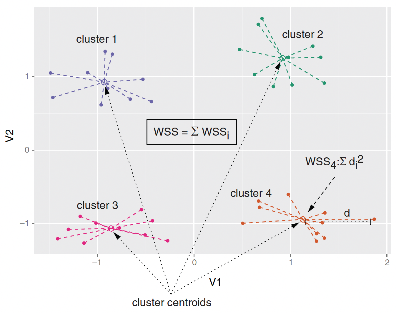
- Ward’s method starts out with each data point as an individual cluster and merges clusters iteratively so as to minimize the total within sum of squares (WSS) of the clustering
🔪 Hierarchical Clustering — Cutting the Tree
cutree() extracts the members of each cluster from the hclust object.
groups_hc <- cutree(pfit, k = 5)

# Convenience function: print selected columns by cluster
print_clusters <- function(data, groups, columns) {
  grouped <- split(data, groups)
  lapply(grouped, function(df) df[, columns])
}

cols_to_print <- c("Country", "RedMeat", "Fish", "FrVeg")
print_clusters(protein, groups_hc, cols_to_print)
🔭 Principal Component Analysis (PCA)
- We can visualize the clustering by projecting the data onto the first two principal components of the data.
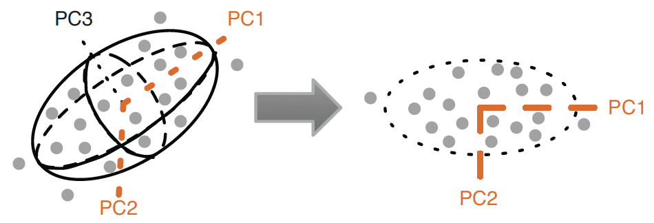
- Ellipsoid is described by three principal components.
- The ellipsoid roughly bounds the data.
- The first two principal components, \(\text{PC}_{1}\) & \(\text{PC}_{2}\), describe the best 2-D projection of the data.
- Notice that the principal components are orthogonal.
- \(Cor(\text{PC}_{1}, \text{PC}_{2}) = 0\)!
🔄 PCA — Rotation and Interpretation
Rotation and interpretation
- Principal components are unknown but associated with variables in the data.
- A principal component can be interpreted in terms of how much each variable in the data is associated with each principal component.
- Principal components describe the data by projecting the data into the space of the (independent) principal components, which is called rotations.
- The maximum number of principal components of the data is the number of numeric variables in the data.
⚙️ PCA — Decomposition
The prcomp() function does the principal components decomposition.
🧩 PC Interpretation — Protein Data

- \(PC_{1}\) is high nut/grain and low meat/dairy:
- \(PC_{1}\) increases by 0.42 with 1 S.D. increase in nuts.
- \(PC_{1}\) decreases by 0.30 with 1 S.D. increase in red meat.
- \(PC_{2}\) is Iberian:
- \(PC_{2}\) increases by 0.65 with 1 S.D. extra fish.
📖 How to Read Loadings — A Simple Rule
The loading table (princ$rotation) shows how much each variable contributes to each PC.
- Large positive loading → variable pulls the PC up (positively associated).
- Large negative loading → variable pulls the PC down (negatively associated).
- Near zero → variable barely contributes to that PC.
- The sign alone doesn’t matter — what matters is which variables have the largest absolute loadings and share the same sign.
- Name the PC by describing what is high vs. low:
- PC1: high Nuts/FrVeg/Cereals vs. low RedMeat/Milk → “Plant-heavy diet”
- PC2: high Fish/Starch vs. low WhiteMeat/FrVeg → “Iberian/coastal diet”
🗺️ PCA Projection by Ward Clusters
ggplot(project_plus, aes(x = PC1, y = PC2)) +
geom_point(data = as.data.frame(project),
color = "darkgrey",
alpha = 0.4) +
geom_point(aes(color = cluster)) +
geom_text(aes(label = country),
hjust = 0, vjust = 1,
size = 3) +
facet_wrap(~ cluster,
ncol = 3, labeller = label_both) +
labs(title = "PCA Projection by Ward Clusters") +
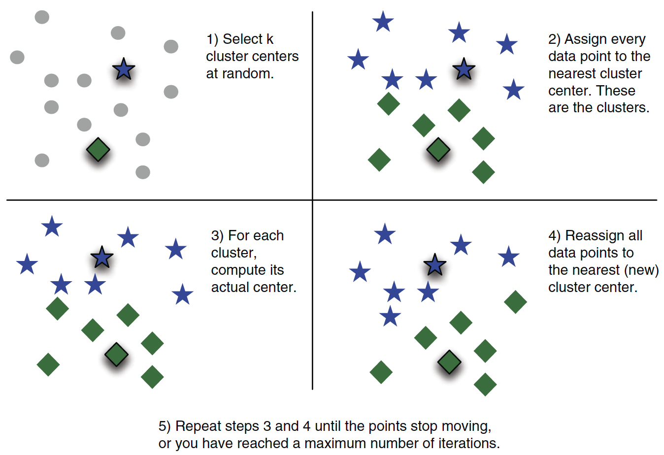
theme(legend.position = "none")🎯 K-means Algorithm
K-Means partitions data into \(k\) groups by assigning each point to the nearest cluster center and iteratively updating the centers to minimize within-cluster variance.
💻 K-means — R Implementation
kmeans() function implements the k-means algorithm.
🏆 Best Number of Clusters — Indices
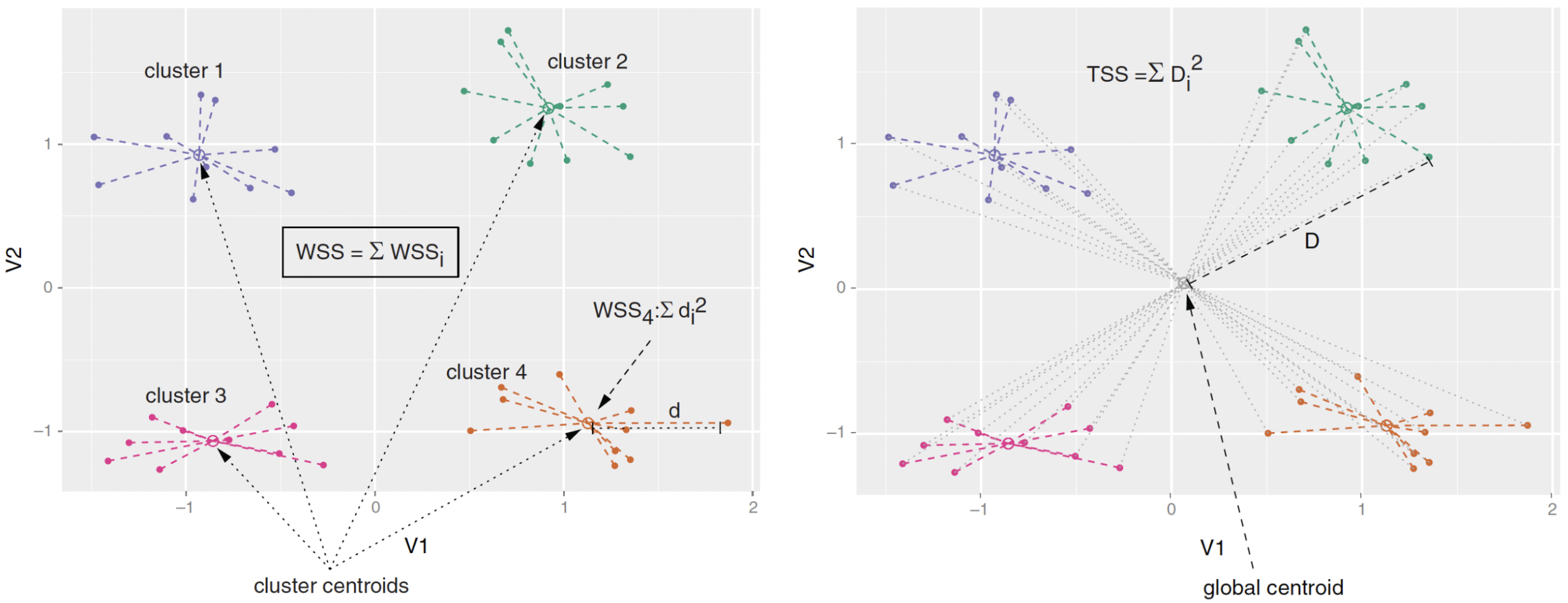
- Calinski-Harabasz Index: the adjusted ratio of between-sum-of-square (BSS) to within-sum-of-square (WSS).
- \(\text{BSS} = \text{TSS} - \text{WSS}\), where \(\text{TSS}\) is total-sum-of-square.
- Good clustering: a small average WSS & a large average BSS.
- Average Silhouette Width (ASW) Index: the mean of individual silhouette coefficients
- Silhouette coefficient quantifies how well a point sits in its cluster by comparing cohesion (avg distance to points in same cluster) and separation (avg distance to points in nearest other cluster).
🔢 Best Number of Clusters — kmeansruns()
The fpc package provides kmeansruns(), which calls kmeans() over a range of \(k\) and selects the best \(k\) automatically.
clustering_ch  <- kmeansruns(pmatrix, krange = 1:10, criterion = "ch")
clustering_asw <- kmeansruns(pmatrix, krange = 1:10, criterion = "asw")

clustering_ch$bestk   # best k by Calinski-Harabasz
clustering_asw$bestk  # best k by Average Silhouette Width

clustering_ch$crit    # criterion scores for each k (CH)
clustering_asw$crit # criterion scores for each k (ASW)- The \(k^{*} = 2\) clustering corresponds to the first split of the protein data dendrogram.
- Clustering with \(k^{*} = 2\) might not be so informative.
📈 Visualizing Cluster Quality — Elbow Plot
The elbow plot shows WSS for each \(k\). Look for the “elbow” where adding more clusters stops improving fit much.
- The x-axis is the number of clusters \(k\).
- The y-axis is total WSS.
- Choose \(k\) at the “elbow” — where the curve bends sharply and flattens out.
- There is no single correct answer; look for the point of diminishing returns.
🗺️ Visualizing K-means Clusters — fviz_cluster()
fviz_cluster() from factoextra projects clusters onto the first two PCs and draws confidence ellipses automatically.
- Points colored by cluster; ellipses show the convex hull of each group.
- Axes are PC1 and PC2 — they explain the largest fraction of variance.
- Use
ellipse.type = "norm"for elliptical confidence regions instead.
📊 Visualizing K-means Clusters — fviz_nbclust() ASW
fviz_nbclust() can also plot the average silhouette width across values of \(k\).
- The peak of this curve is the recommended \(k\).
- Compare with the elbow plot and dendrogram to arrive at a final choice.
📺 NBC Show Data
- Data from NBC on response to TV pilots
- Gross Ratings Points (GRP): estimated total viewership, which measures broadcast marketability.
- Projected Engagement (PE): a more subtle measure of audience.
- After watching a show, viewer is quizzed on order and detail.
- This measures their engagement with the show (and ads!).
url_shows <- "https://bcdanl.github.io/data/nbc_show.csv"
shows <- read_csv(url_shows) |>
  mutate(Genre = as.factor(Genre))

ggplot(shows, aes(x = GRP, y = PE, color = Genre)) +
  geom_point(size = 2.5, alpha = 0.8) +
  geom_smooth(method = "lm", se = FALSE, linewidth = 0.8) +
  labs(title = "Gross Rating Points vs. Projected Engagement")
📋 NBC Show Survey
- After watching a show, viewer is quizzed on order and detail.
- The survey data include 6241 views and 20 questions for 40 shows.
- There are two types of questions in the survey.
- For Q1, this statement takes the form of “This show makes me feel …”
- For Q2, the statement is “I find this show feel …”
- To relate survey results to show performance, we first calculate the average survey response by show.
url_survey <- "https://bcdanl.github.io/data/nbc_survey.csv"
survey <- read_csv(url_survey)

# Average each question by show, then align row order to shows
pilot_avg <- survey |>
  select(-Viewer) |>
  group_by(Show) |>
  summarise(across(everything(), mean)) |>
  filter(Show %in% shows$Show) |>
  arrange(match(Show, shows$Show)) |>
  column_to_rownames("Show")
📉 Scree Plot
The scree plot is simply showing us, for each principal component \(j\) (on the \(x\)-axis), what fraction of the total variance in our pilot-survey data that component captures (on the \(y\)-axis).
\[ Var(PC_{1}) \geq Var(PC_{2}) \geq Var(PC_{3}) \geq \cdots \]
📖 How to Read a Scree Plot
- The y-axis shows percent of variance explained by each PC.
- The x-axis is the index of each principal component.
- Key reading rules:
Look for the “elbow”:
- The variance drops steeply at first, then levels off.
- Keep PCs before the elbow — they capture most of the signal.
- PCs after the elbow mostly capture noise.
- In the NBC survey, PC1 + PC2 together explain the bulk of variation → we use 2 PCs.
🔍 PC Interpretation — NBC Survey
- \(\text{PC}_{1}\) (“Overall Engagement”)
- \(\text{PC}_{2}\) (“Passive/Comfort vs. Active Drama”)
📖 Reading NBC Loadings Step by Step
Use the same three-step process for any PCA loading table:
- Find the largest absolute values in each row (PC).
- Note the sign — positive means the variable raises that PC, negative means it lowers it.
- Name the PC by describing the contrast (what is high vs. low).
- PC1 — large positive loadings on all Q1/Q2 items → represents overall engagement level.
- Shows with high PC1 score = viewers felt high engagement across all questions.
- PC2 — positive loadings on comfort/passive feelings, negative on drama/tension items.
- Shows with high PC2 = comfort/relaxing content; low PC2 = intense/dramatic content.
🌐 PCA Projection of NBC Shows
Z <- predict(princ_nbc, X)

zpilot_df <- as.data.frame(Z[, 1:2]) |>
  mutate(Show  = shows$Show,
         Genre = shows$Genre,
         PE    = shows$PE,
         GRP   = shows$GRP,
         PE_norm = (PE - min(PE)) / (max(PE) - min(PE)))

ggplot(zpilot_df, aes(x = PC1, y = PC2, color = Genre, size = PE_norm)) +
  geom_point(alpha = 0.5) +
  geom_text(aes(label = Show), size = 2.5, hjust = 0, vjust = 1,
            show.legend = FALSE) +
  scale_size_continuous(range = c(2, 10), name = "PE (normalized)") +
  labs(title = "NBC Pilots in Survey PC Space")
📖 Principal Component Regression (PCR)
- PCR uses a lower-dimension set of principal components as predictors.
- PC analysis can reduce dimension, which is usually good.
- The PCs are independent (\(Cov(PC_{i}, PC_{j}) = 0\)).
- PC analysis will be driven by the dominant sources of variation in \(x\).
- If the outcome is connected to these dominant sources of variation, PCR works well.
- The AIC (Akaike information criterion) is negatively associated to the probability that the data would be observed from the model.
- The lower AIC is, the better model is.
💡 PCR — Model Selection by AIC
max_K    <- min(20, ncol(Z))
aic_pe   <- numeric(max_K)
aic_grp  <- numeric(max_K)

for (k in seq_len(max_K)) {
  Xk          <- cbind(1, Z[, 1:k])           # intercept + first k PCs
  aic_pe[k]   <- AIC(lm(shows$PE  ~ Z[, 1:k]))
  aic_grp[k]  <- AIC(lm(shows$GRP ~ Z[, 1:k]))
}

cat("Lowest AIC for PE  achieved with K =", which.min(aic_pe),  "PCs\n")
cat("Lowest AIC for GRP achieved with K =", which.min(aic_grp), "PCs\n")
📈 PCR — AIC Plot
tibble(K = 1:max_K, PE = aic_pe, GRP = aic_grp) |>
  pivot_longer(c(PE, GRP), names_to = "Outcome", values_to = "AIC") |>
  ggplot(aes(x = K, y = AIC, color = Outcome)) +
  geom_line() + geom_point() +
  facet_wrap(~Outcome, ncol = 1, scales = "free") +
  scale_x_continuous(breaks = 1:max_K) +
  labs(title = "PCR Model Comparison: AIC vs. Number of Principal Components",
       x = "Number of Principal Components (K)", y = "AIC")
🗺️ Full Workflow Summary
🗺️ Full Clustering + PCA Workflow
Every clustering + PCA analysis follows the same pipeline. Follow this order:
# ── STEP 1: Load data ──────────────────────────────────────────────────────
df <- read_csv("YOUR_DATA.csv")

# ── STEP 2: Scale numeric variables ────────────────────────────────────────
vars    <- colnames(df)[-1]          # drop ID/label column
mat     <- scale(df[, vars])         # mean=0, sd=1
rownames(mat) <- df$ID_column        # label rows for dendrograms

# ── STEP 3a: Hierarchical clustering ───────────────────────────────────────
distmat <- dist(mat, method = "euclidean")
hfit    <- hclust(distmat, method = "ward.D")
fviz_dend(hfit, k = 5, rect = TRUE)  # choose k visually

# ── STEP 3b: Cut the tree to get cluster labels ─────────────────────────────
groups_hc <- cutree(hfit, k = 5)

# ── STEP 4: Choose k for k-means (elbow + silhouette) ──────────────────────
fviz_nbclust(mat, kmeans, method = "wss")
fviz_nbclust(mat, kmeans, method = "silhouette")
kmeansruns(mat, krange = 1:10, criterion = "ch")$bestk
kmeansruns(mat, krange = 1:10, criterion = "asw")$bestk

# ── STEP 5: K-means ─────────────────────────────────────────────────────────
km  <- kmeans(mat, centers = 5, nstart = 100, iter.max = 100)
fviz_cluster(km, data = mat, geom = c("point","text"), repel = TRUE)

# ── STEP 6: PCA ──────────────────────────────────────────────────────────────
pc  <- prcomp(mat)
fviz_eig(pc, addlabels = TRUE)       # scree plot
t(round(pc$rotation, 2))[1:2, ]     # loadings

# ── STEP 7: PCA projection coloured by cluster ─────────────────────────────
proj <- as.data.frame(predict(pc, mat)[, 1:2])
proj$cluster <- as.factor(groups_hc)
ggplot(proj, aes(x = PC1, y = PC2, color = cluster)) + geom_point()
✅ Step-by-Step Checklist
Use this checklist every time you run a clustering + PCA analysis:
| Step | Action | Key function |
|---|---|---|
| 1 | Load data | read_csv() |
| 2 | Scale numeric variables | scale() |
| 3 | Build dendrogram | hclust() + fviz_dend() |
| 4 | Cut tree | cutree(fit, k = K) |
| 5 | Choose k (elbow) | fviz_nbclust(..., method="wss") |
| 6 | Choose k (silhouette) | fviz_nbclust(..., method="silhouette") |
| 7 | Run k-means | kmeans(mat, K, nstart=100) |
| 8 | Visualize clusters | fviz_cluster() |
| 9 | Run PCA | prcomp(mat) |
| 10 | Scree plot | fviz_eig() |
| 11 | Read loadings | t(round(pc$rotation, 2)) |
| 12 | Project + color by cluster | predict(pc, mat) + ggplot() |
🧠 Common Questions on Interpretation - 1
- Q: How do I name a principal component?
- Look at the two or three variables with the largest absolute loading values.
- Describe what is high (large positive) versus low (large negative) on that PC.
- Example: PC1 has large positive loading on
Fishand large negative onRedMeat→ “Fish-heavy vs. meat-heavy diet.”
- Q: How many PCs should I keep?
- Use the scree plot elbow: keep PCs before the curve flattens.
- Or use the cumulative variance rule: keep enough PCs to explain ≥ 70–80% of variance.
summary(prcomp_object)$importanceshows cumulative proportions.
🧠 Common Questions on Interpretation - 2
- Q: Which k to choose for k-means?
- Look at the elbow plot (WSS), the silhouette plot (ASW), and the dendrogram.
- If they agree → use that \(k\). If they disagree → use subject-matter knowledge or interpretability.
- Q: What is
fviz_cluster()actually plotting?- It projects the data onto PC1 and PC2 and colors points by cluster label. The axis labels tell you how much variance each PC explains.