Lecture 7

Linear Regression

Byeong-Hak Choe

bchoe@geneseo.edu

SUNY Geneseo

February 17, 2025

Big Data and Machine Learning

Big Data and Machine Learning (ML)

• The term “Big Data” originated from computer scientists working with datasets too large to fit on a single machine.
  • As aggregation evolved into analysis, Big Data became closely linked with statistics and machine learning (ML).
  • Scalability of algorithms is crucial for handling large datasets.
• We will use ML to:
  ✅ Identify patterns in big data
  ✅ Make data-driven decisions

What does it mean to be “big”?

• Big in both the number of observations (size n) and in the number of variables (dimension p).

• In these settings, we cannot:

  • Look at each individual variable and make a decision.
  • Choose among a small set of candidate models.
  • Plot every variable to look for interactions or transformations.

• Some ML tools are straight out of previous statistics classes (linear regression) and some are totally new (ensemble models, principal component analysis).

  • All require a different approach when n and p get really big.

ML topics

• Regression: inference and prediction
• Regularization: cross-validation
• Principal Component Analysis: dimension reduction
• Tree-based models: decision trees, random forest, XGBoost
• Classfication: kNN
• Clustering: k-means, association rules
• Text Mining: sentiment analysis; topic models

Linear Regression Model

Models and Assumptions

Linear Model

• Linear regression assumes a linear relationship for \(Y = f(X_{1})\):

\[Y_{i} \,=\, \beta_{0} \,+\, \beta_{1} X_{1, i} \,+\, \epsilon_{i}\] for \(i \,=\, 1, 2, \dots, n\), where \(i\) is the \(i\)-th observation in data.

• \(Y_i\) is the \(i\)-th value for the outcome/dependent/response/target variable \(Y\).

• \(X_{1, i}\) is the \(i\)-th value for the explanatory/independent/predictor/input variable or feature \(X_{1}\).

Models and Assumptions

Beta coefficients

• Linear regression assumes a linear relationship for \(Y = f(X_{1})\):

\[Y_{i} \,=\, \beta_{0} \,+\, \beta_{1} X_{1, i} \,+\, \epsilon_{i}\] for \(i \,=\, 1, 2, \dots, n\), where \(i\) is the \(i\)-th observation in data.

• \(\beta_0\) is an unknown true value of an intercept: average value for \(Y\) if \(X_{1} = 0\)

• \(\beta_1\) is an unknown true value of a slope: increase in average value for \(Y\) for each one-unit increase in \(X_{1}\)

Models and Assumptions

Random Noises

• Linear regression assumes a linear relationship for \(Y = f(X_{1})\):

\[Y_{i} \,=\, \beta_{0} \,+\, \beta_{1} X_{1, i} \,+\, \epsilon_{i}\] for \(i \,=\, 1, 2, \dots, n\), where \(i\) is the \(i\)-th observation in data.

• \(\epsilon_i\) is a random noise, or a statistical error:

\[ \epsilon_i \sim N(0, \sigma^2) \]

• Errors have a mean value of 0 with constant variance \(\sigma^2\).
• Errors are uncorrelated with \(X_{1, i}\).

What Is Linear Regression Doing?

Best Fitting Line

• Linear regression finds the beta estimates \(( \hat{\beta_{0}}, \hat{\beta_{1}} )\) such that:

  – The linear function \(f(X_{1}) = \hat{\beta_{0}} + \hat{\beta_{1}}X_{1}\) is as near as possible to \(Y\) for all \((X_{1, i}\,,\, Y_{i})\) pairs in the data.

  • It is the best fitting line, or the predicted outcome, \(\hat{Y_{\,}} = \hat{\beta_{0}} + \hat{\beta_{1}}X_{1}\).

What Is Linear Regression Doing?

Residual errors

• The estimated beta coefficients are chosen to minimize the sum of squares of the residual errors \((SSR)\): \[ \begin{align} SSR &\,=\, (\texttt{Residual_Error}_{1})^{2}\\ &\quad \,+\, (\texttt{Residual_Error}_{2})^{2}\\ &\quad\,+\, \cdots + (\texttt{Residual_Error}_{n})^{2}\\ \text{where}\qquad\qquad\qquad\qquad&\\ \texttt{Residual_Error}_{i} &\,=\, Y_{i} \,-\, \hat{Y_{i}},\\ \texttt{Predicted_Outcome}_{i}: \hat{Y_{i}} &\,=\, \hat{\beta_{0}} \,+\, \hat{\beta_{1}}X_{1, i} \end{align} \]

What Is Linear Regression Doing?

Hat Notation

• We use the hat notation \((\,\hat{\texttt{ }_{\,}}\,)\) to distinguish true values and estimated/predicted values.

• The value of true beta coefficient is denoted by \(\beta_{1}\).

• The value of estimated beta coefficient is denoted by \(\hat{\beta_{1}}\).

• The \(i\)-th value of true outcome variable is denoted by \(Y_{i}\).

• The \(i\)-th value of predicted outcome variable is denoted by \(\hat{Y_{i}}\).

What Is Linear Regression Doing?

Relationship

1. Finding the relationship between \(X_{1}\) and \(Y\) \[\hat{\beta_{1}}\]: How is an increase in \(X_1\) by one unit associated with a change in \(Y\) on average? - Positive? Negative? Independent? - How strong?

Statistical Significance in Estimated Beta Coefficients

• What does it mean for a beta estimate \(\hat{\beta_{\,}}\) to be statistically significant at 5% level?
  • It means that the null hypothesis \(H_{0}: \beta = 0\) is rejected for a given significance level 5%.
  • “2 standard error rule” of thumb: The true value of \(\beta\) is 95% likely to be in the confidence interval \((\, \hat{\beta_{\,}} - 2 * \texttt{Std. Error}\;,\; \hat{\beta_{\,}} + 2 * \texttt{Std. Error} \,)\).
  • The standard error tells us how uncertain our beta estimate is.
  • We should look for the stars!

What Is Linear Regression Doing?

Prediction

2. Making a prediction on \(Y\): \[\hat{Y_{\,}}\] For unseen data point of \(X_1\), what is the predicted value of outcome, \(\hat{Y_{\,}}\)?

• E.g., For \(X_{1} = 2\), the predicted outcome is \(\hat{Y_{\,}} = \hat{\beta_{0}} + \hat{\beta_{1}} \times 2\).
• E.g., For \(X_{1} = 3\), the predicted outcome is \(\hat{Y_{\,}} = \hat{\beta_{0}} + \hat{\beta_{1}} \times 3\).

Linear Regression - Example

• Suppose we want to predict a property’s sales price based on the property size.
  • In other words, for some house sale i, we want to predict sale_price[i] based on gross_square_feet[i].
• We also want to focus on the relationship between a property’s sales price and a property size.
  • In other words, we estimate how an increase in gross_square_feet[i] is associated with sale_price[i].

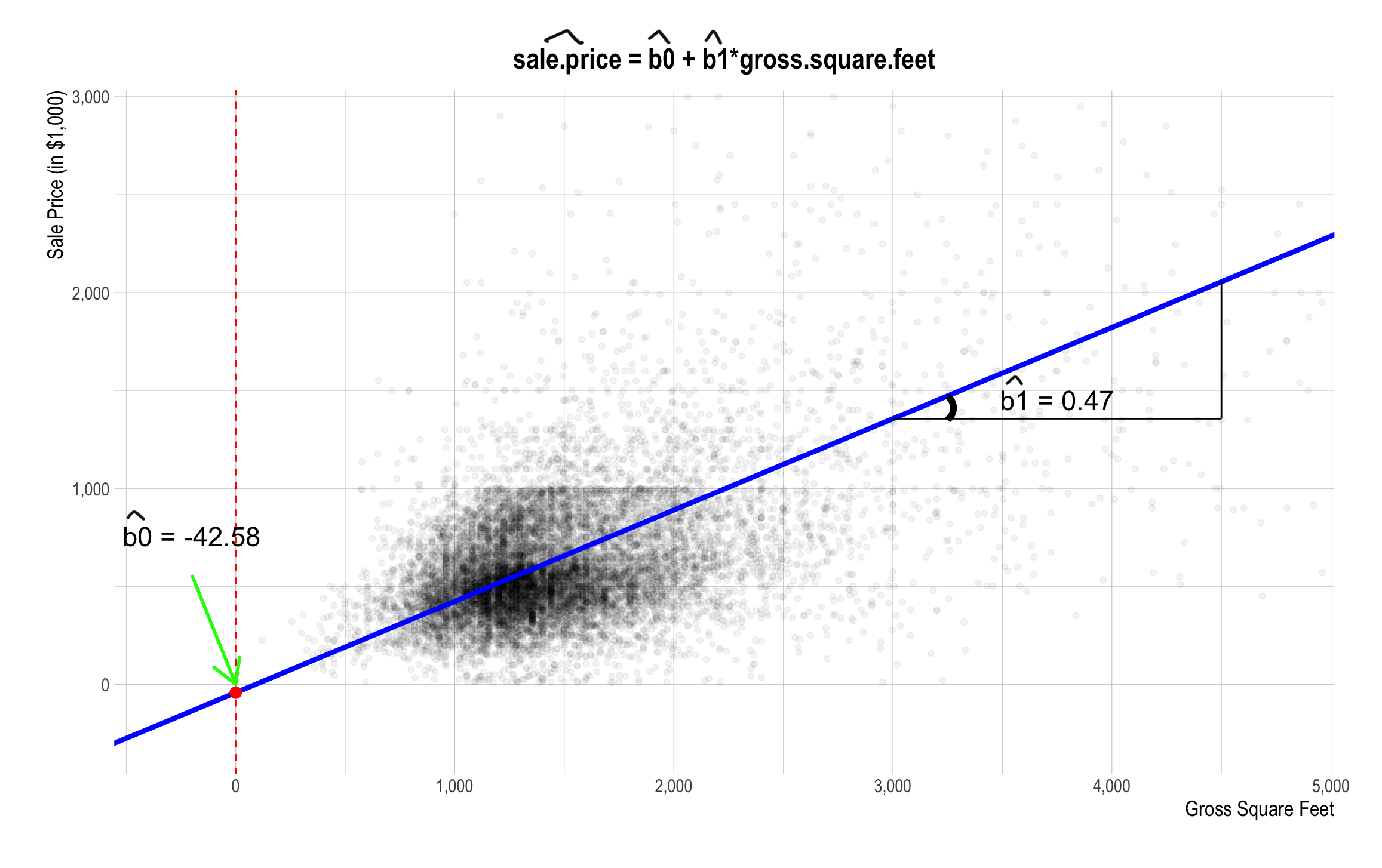
Linear Relationship

• Linear regression assumes that:

  • The outcome sale_price[i] is linearly related to the input gross_square_feet[i]:

\[\texttt{sale_price[i]} \;=\quad \texttt{b0} \,+\, \texttt{b1*gross_square_feet[i]} \,+\, \texttt{e[i]}\] where e[i] is a statistical error term.

The Linear Relationship between sale_price and gross_square_feet

Best Fitting Line

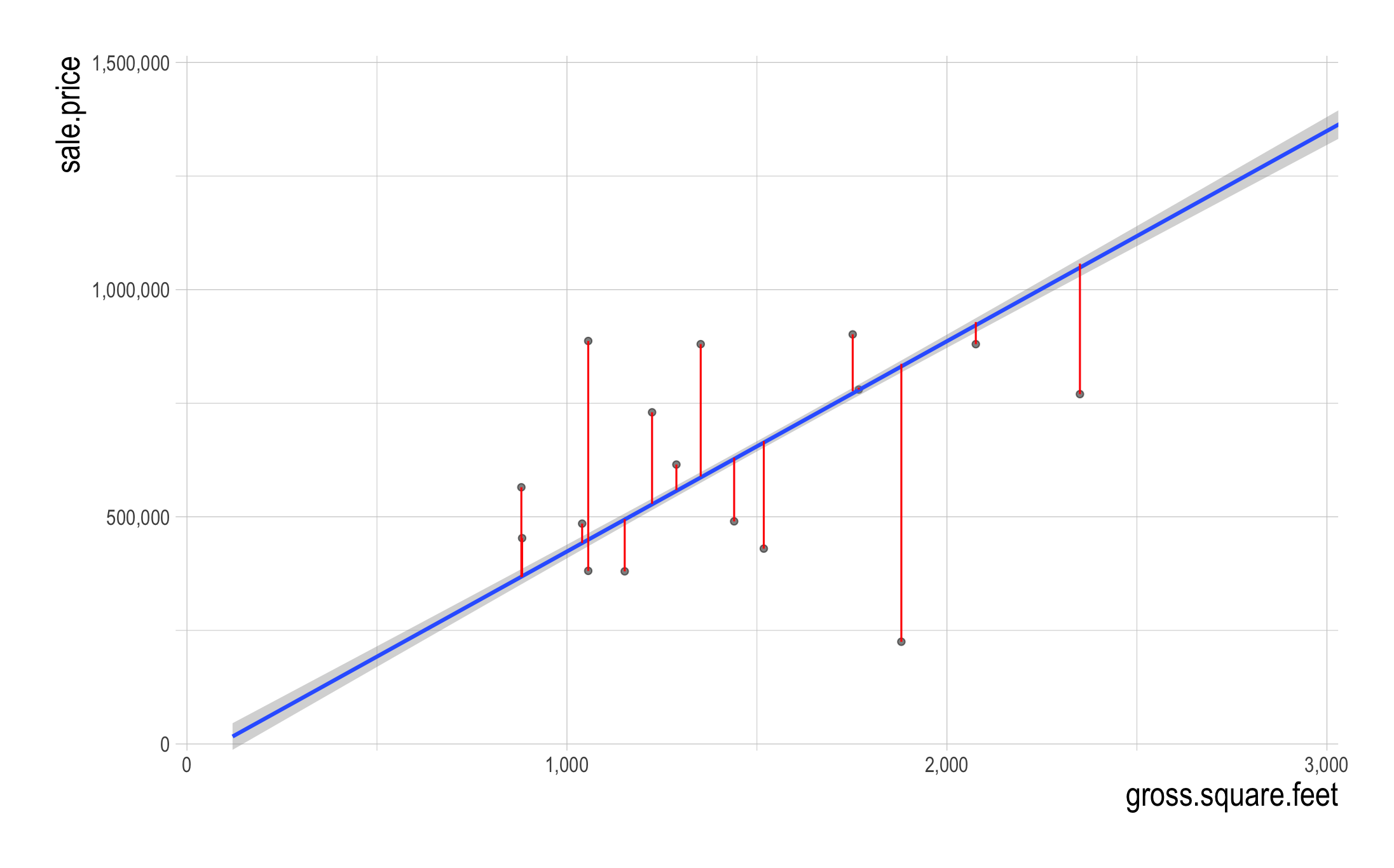
• What do the vertical lines visualize?

Model Evaluation

Mean squared error (MSE)

• One of the most common metrics used to measure the prediction accuracy of a linear regression model is MSE, which stands for mean squared error.
  • \(MSE\) is \(SSR\) divided by \(n\) (the number of observations in the data that are used in making predictions).

\[ MSE = SSR / n \] \[ \begin{align} SSR &\,=\, (\texttt{Residual_Error}_{1})^{2}\\ &\quad \,+\, (\texttt{Residual_Error}_{2})^{2}\\ &\quad\,+\, \cdots + (\texttt{Residual_Error}_{n})^{2} \end{align} \]

• The lower MSE, the higher accuracy of the model.
  
• The root MSE (RMSE) is the square root of MSE.

Model Evaluation

Mean squared error (MSE)

• The root MSE (RMSE) represents the overall deviation of \(Y_{i}\) from the best fitting regression line.

Model Evaluation

R-squared

• R-squared is a measure of how well the model “fits” the data, or its “goodness of fit.”

  • R-squared can be thought of as what fraction of the y’s variation is explained by the explanatory variables.

• We want R-squared to be fairly large and R-squareds that are similar on testing and training.

• Caution: R-squared will be higher for models with more explanatory variables, regardless of whether the additional explanatory variables actually improve the model or not.

Goals of Linear Regression

• The goals of linear regression here are to:

1. Modeling for explanation: Find the relationship between gross_square_feet and sale_price by estimating a true value of b1.

• The estimated value of b1 is denoted by \(\hat{\texttt{b1}}\).

2. Modeling for prediction: Make a prediction on sale_price[i] for new property i

• The predicted value of sale_price[i] is denoted by \(\widehat{\texttt{sale_price}}\texttt{[i]}\), where

\[\widehat{\texttt{sale_price}}\texttt{[i]} \;=\quad \hat{\texttt{b0}} \,+\, \hat{\texttt{b1}}\texttt{*gross_square_feet[i]}\]

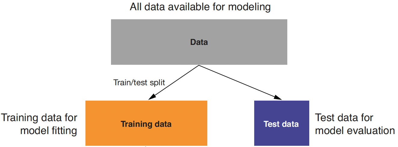
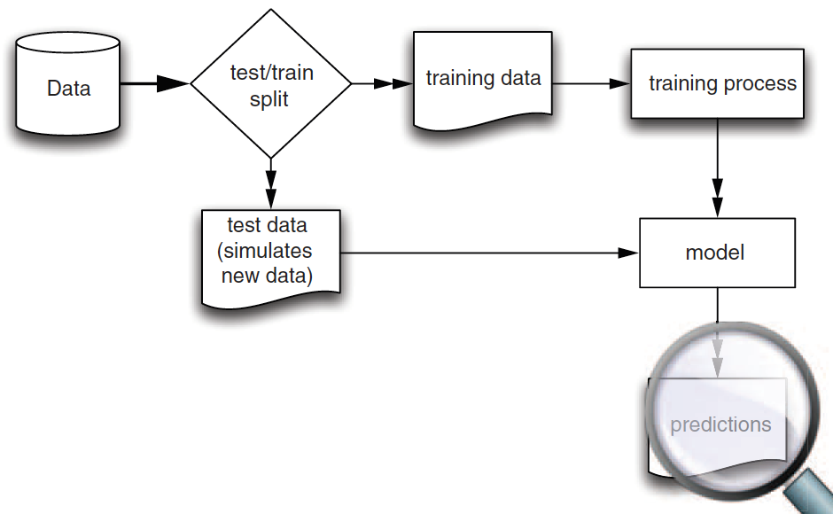
Training and Test Data

• Training data: When we’re building a linear regression model, we need data to train the model.

• Test data: We also need data to test whether the model works well on new data.

• So, we start with splitting a given data.frame into training and test data.frames when building a linear regression model.

Training and Test Data

Training vs. Test

• We use training data to train/fit the linear regression model.
  • We then make a prediction using test data, which are unseen/new from the viewpoint of the trained linear regression model.
• In this way, we can test whether our model performs well in the real world, where unseen data points exist.

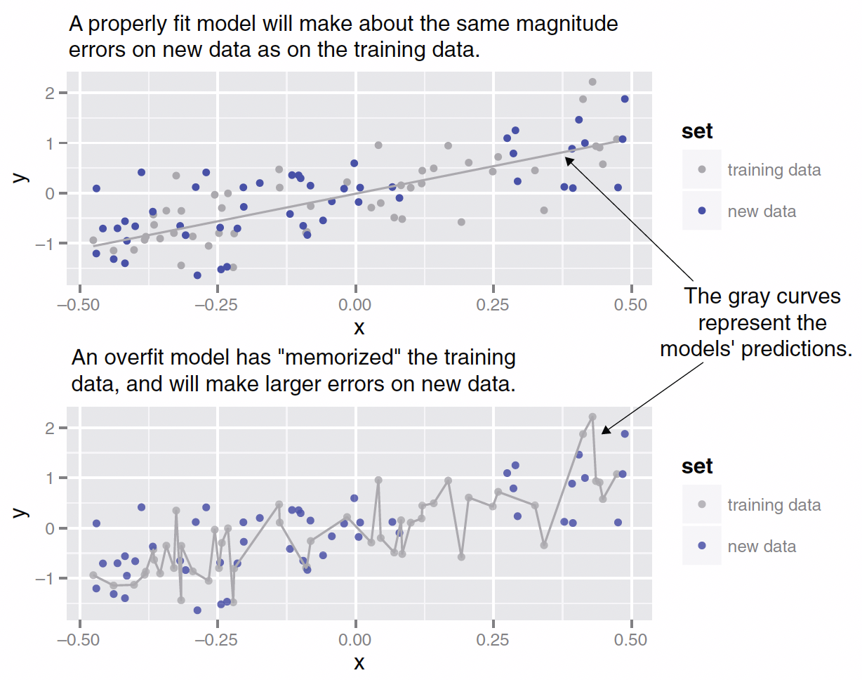
Training and Test Data

Overfitting

Training and Test Data

Model Construction and Evaluation

Splitting Data into Training and Testing Data

A Little Bit of Statistics for the Uniform Distribution

• The probability density function for the uniform distribution looks like:

• With the uniform distribution, any values of \(x\) between 0 and 1 is equally likely drawn.

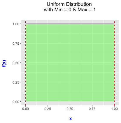
• We will use the uniform distribution when splitting data into training and testing data sets.

Splitting Data into Training and Testing Data

Randomization in the Sampling Process

• Why do we randomize when splitting given data into training and test data?
  • Randomizing the sampling process ensures that the training and test data sets are representative for the population data.
  • If the sample does not properly represent the entire population, the model result is biased toward the sample.
• Suppose the splitting process is not randomized, so that the observations with sale_price > 10^6 are in the training data and the observations with sale_price <= 10^6 are in the test data.
  • What would be the model result then?

Linear Regression using PySpark

Example of Linear Regression using PySpark

• We will use the data for residential property sales from September 2017 and August 2018 in NYC.

• Each sales data recorded contains a number of interesting variables, but here we focus on the followings:

  • sale_price: a property’s sales price;
  • gross_square_feet: a property’s size;
  • age: a property’s age;
  • borough_name: a borough where a property is located.

• Use summary statistics and visualization to explore the data.

Splitting Data into Training and Testing Data

Step 1. Importing Modules and Reading DataFrames

import pandas as pd
import numpy as np
from tabulate import tabulate  # for table summary
import scipy.stats as stats
import matplotlib.pyplot as plt
import seaborn as sns
import statsmodels.api as sm  # for lowess smoothing

from pyspark.sql import SparkSession
from pyspark.sql.functions import rand, col, pow, mean, avg, when, log, sqrt
from pyspark.ml.feature import VectorAssembler
from pyspark.ml.regression import LinearRegression

spark = SparkSession.builder.master("local[*]").getOrCreate()

# 1. Read CSV data from URL
df_pd = pd.read_csv('https://bcdanl.github.io/data/home_sales_nyc.csv')
sale_df = spark.createDataFrame(df_pd)
sale_df.show()

Splitting Data into Training and Testing Data

Step 2. rand(seed = ANY_NUMBER)

# 2. Split data into training and testing sets by creating a random column "gp"
sale_df = sale_df.withColumn("gp", rand(seed=123)) # seed is set for replication

# Splits 60-40 into training and test sets 
dtrain = sale_df.filter(col("gp") >= 0.4) 
dtest = sale_df.filter(col("gp") < 0.4)

# Or simply,
dtrain, dtest = sale_df.randomSplit([0.6, 0.4], seed = 123)

Building an ML DataFrame using VectorAssembler()

# Now assemble predictors using the renamed column
assembler1 = VectorAssembler(
    inputCols=["gross_square_feet"], 
    outputCol="predictors")

• VectorAssembler is a transformer in PySpark’s ML library that is used to combine multiple columns into a single vector column.
  • Many ML algorithms in Spark require the predictors to be represented as a single vector.
  • VectorAssembler is often one of the first steps in a Spark ML pipeline.

Building an ML DataFrame using VectorAssembler()

dtrain1 = assembler1.transform(dtrain) # training data
dtest1  = assembler1.transform(dtest)  # test data

dtrain1.select("predictors", "sale_price").show()
dtest1.select("predictors", "sale_price").show()

• VectorAssembler.transform() returns a DataFrame with a new column, specified in outputCol in VectorAssembler().

Building a Linear Regression Model using LinearRegression().fit()

# Fit linear regression model using the new label column "sale_price"
model1 = (
    LinearRegression(
        featuresCol = "predictors", 
        labelCol = "sale_price")
    .fit(dtrain1)
)

• LinearRegression(featuresCol="predictors", labelCol="sale_price")
  • This creates an instance of the LinearRegression class.
  • The features (independent variables) are in a column named “predictors”.
  • The label (dependent variable) is in a column named “sale_price”.
• .fit() trains (fits) the linear regression model using the training DataFrame dtrain1.
  • This training process estimates the beta coefficients that best predict the label from the features.

Building a Linear Regression Model using LinearRegression().fit()

# Adding a "prediction" coulmn to dtest1 DataFrame
dtest1  = model1.transform(dtest1)

• dtest1 = model1.transform(dtest1): Adds a new column prediction to dtest1 DataFrame.
  • This new column contains the predicted outcome based on the trained model1 to predict an outcome for the test dataset dtest1.

Summary of the Regression Result

model1.intercept
model1.coefficients
model1.summary.coefficientStandardErrors
model1.summary.rootMeanSquaredError
model1.summary.r2

Summary of the Regression Result

Example of a Regression Table

Summary of the Regression Result

Make the Summary Pretty

def regression_table(model, assembler):
    """
    Creates a formatted regression table from a fitted LinearRegression model and its VectorAssembler.

    If the model’s labelCol (retrieved using getLabelCol()) starts with "log", an extra column showing np.exp(coeff)
    is added immediately after the beta estimate column for predictor rows. Additionally, np.exp() of the 95% CI
    Lower and Upper bounds is also added unless the predictor's name includes "log_". The Intercept row does not
    include exponentiated values.

    When labelCol starts with "log", the columns are ordered as:
        y: [label] | Beta | Exp(Beta) | Sig. | Std. Error | p-value | 95% CI Lower | Exp(95% CI Lower) | 95% CI Upper | Exp(95% CI Upper)

    Otherwise, the columns are:
        y: [label] | Beta | Sig. | Std. Error | p-value | 95% CI Lower | 95% CI Upper

    Parameters:
        model: A fitted LinearRegression model (with a .summary attribute and a labelCol).
        assembler: The VectorAssembler used to assemble the features for the model.

    Returns:
        A formatted string containing the regression table.
    """
    # Determine if we should display exponential values for coefficients.
    is_log = model.getLabelCol().lower().startswith("log")

    # Extract coefficients and standard errors as NumPy arrays.
    coeffs = model.coefficients.toArray()
    std_errors_all = np.array(model.summary.coefficientStandardErrors)

    # Check if the intercept's standard error is included (one extra element).
    if len(std_errors_all) == len(coeffs) + 1:
        intercept_se = std_errors_all[0]
        std_errors = std_errors_all[1:]
    else:
        intercept_se = None
        std_errors = std_errors_all

    # Use provided tValues and pValues.
    df = model.summary.numInstances - len(coeffs) - 1
    t_critical = stats.t.ppf(0.975, df)
    p_values = model.summary.pValues

    # Helper: significance stars.
    def significance_stars(p):
        if p < 0.01:
            return "***"
        elif p < 0.05:
            return "**"
        elif p < 0.1:
            return "*"
        else:
            return ""

    # Build table rows for each feature.
    table = []
    for feature, beta, se, p in zip(assembler.getInputCols(), coeffs, std_errors, p_values):
        ci_lower = beta - t_critical * se
        ci_upper = beta + t_critical * se

        # Check if predictor contains "log_" to determine if exponentiation should be applied
        apply_exp = is_log and "log_" not in feature.lower()

        exp_beta = np.exp(beta) if apply_exp else ""
        exp_ci_lower = np.exp(ci_lower) if apply_exp else ""
        exp_ci_upper = np.exp(ci_upper) if apply_exp else ""

        if is_log:
            table.append([
                feature,            # Predictor name
                beta,               # Beta estimate
                exp_beta,           # Exponential of beta (or blank)
                significance_stars(p),
                se,
                p,
                ci_lower,
                exp_ci_lower,       # Exponential of 95% CI lower bound
                ci_upper,
                exp_ci_upper        # Exponential of 95% CI upper bound
            ])
        else:
            table.append([
                feature,
                beta,
                significance_stars(p),
                se,
                p,
                ci_lower,
                ci_upper
            ])

    # Process intercept.
    if intercept_se is not None:
        intercept_p = model.summary.pValues[0] if model.summary.pValues is not None else None
        intercept_sig = significance_stars(intercept_p)
        ci_intercept_lower = model.intercept - t_critical * intercept_se
        ci_intercept_upper = model.intercept + t_critical * intercept_se
    else:
        intercept_sig = ""
        ci_intercept_lower = ""
        ci_intercept_upper = ""
        intercept_se = ""

    if is_log:
        table.append([
            "Intercept",
            model.intercept,
            "",                    # Removed np.exp(model.intercept)
            intercept_sig,
            intercept_se,
            "",
            ci_intercept_lower,
            "",
            ci_intercept_upper,
            ""
        ])
    else:
        table.append([
            "Intercept",
            model.intercept,
            intercept_sig,
            intercept_se,
            "",
            ci_intercept_lower,
            ci_intercept_upper
        ])

    # Append overall model metrics.
    if is_log:
        table.append(["Observations", model.summary.numInstances, "", "", "", "", "", "", "", ""])
        table.append(["R²", model.summary.r2, "", "", "", "", "", "", "", ""])
        table.append(["RMSE", model.summary.rootMeanSquaredError, "", "", "", "", "", "", "", ""])
    else:
        table.append(["Observations", model.summary.numInstances, "", "", "", "", ""])
        table.append(["R²", model.summary.r2, "", "", "", "", ""])
        table.append(["RMSE", model.summary.rootMeanSquaredError, "", "", "", "", ""])

    # Format the table rows.
    formatted_table = []
    for row in table:
        formatted_row = []
        for i, item in enumerate(row):
            # Format Observations as integer with commas.
            if row[0] == "Observations" and i == 1 and isinstance(item, (int, float, np.floating)) and item != "":
                formatted_row.append(f"{int(item):,}")
            elif isinstance(item, (int, float, np.floating)) and item != "":
                if is_log:
                    # When is_log, the columns are:
                    # 0: Metric, 1: Beta, 2: Exp(Beta), 3: Sig, 4: Std. Error, 5: p-value,
                    # 6: 95% CI Lower, 7: Exp(95% CI Lower), 8: 95% CI Upper, 9: Exp(95% CI Upper).
                    if i in [1, 2, 4, 6, 7, 8, 9]:
                        formatted_row.append(f"{item:,.3f}")
                    elif i == 5:
                        formatted_row.append(f"{item:.3f}")
                    else:
                        formatted_row.append(f"{item:.3f}")
                else:
                    # When not is_log, the columns are:
                    # 0: Metric, 1: Beta, 2: Sig, 3: Std. Error, 4: p-value, 5: 95% CI Lower, 6: 95% CI Upper.
                    if i in [1, 3, 5, 6]:
                        formatted_row.append(f"{item:,.3f}")
                    elif i == 4:
                        formatted_row.append(f"{item:.3f}")
                    else:
                        formatted_row.append(f"{item:.3f}")
            else:
                formatted_row.append(item)
        formatted_table.append(formatted_row)

    # Set header and column alignment based on whether label starts with "log"
    if is_log:
        headers = [
            f"y: {model.getLabelCol()}",
            "Beta", "Exp(Beta)", "Sig.", "Std. Error", "p-value",
            "95% CI Lower", "Exp(95% CI Lower)", "95% CI Upper", "Exp(95% CI Upper)"
        ]
        colalign = ("left", "right", "right", "center", "right", "right", "right", "right", "right", "right")
    else:
        headers = [f"y: {model.getLabelCol()}", "Beta", "Sig.", "Std. Error", "p-value", "95% CI Lower", "95% CI Upper"]
        colalign = ("left", "right", "center", "right", "right", "right", "right")

    table_str = tabulate(
        formatted_table,
        headers=headers,
        tablefmt="pretty",
        colalign=colalign
    )

    # Insert a dashed line after the Intercept row.
    lines = table_str.split("\n")
    dash_line = '-' * len(lines[0])
    for i, line in enumerate(lines):
        if "Intercept" in line and not line.strip().startswith('+'):
            lines.insert(i+1, dash_line)
            break

    return "\n".join(lines)

# Example usage:
# print(regression_table(model_1, assembler_1))

Summary of the Regression Result

Make the Summary Pretty

# Using the UDF, regression_table(model, assembler)
print(regression_table(model1, assembler1))

Linear Regression Model with Multiple Predictors

Multiple Regression

• What if the regression were missing something?
  • Maybe prices are not just about size, but maybe there are certain parts of NYC that are categorically more expensive than other parts of NYC.
  • Maybe Manhattan is just more expensive than Bronx.
  • Maybe apartments are different than non-apartments.
  • Maybe old houses are different than new houses.
• It is often helpful to bring in multiple explanatory variables—a Multivariate Regression.

Models and Assumptions

• Linear regression assumes a linear relationship for \(Y = f(X_{1}, X_{2})\):

\[Y_{i} \,=\, \beta_{0} \,+\, \beta_{1} X_{1, i} \,+\,\beta_{2} X_{2, i} \,+\, \epsilon_{i}\] for \(i \,=\, 1, 2, \dots, n\), where \(i\) is the \(i\)-th observation in data.

• \(\beta_0\) is an unknown true value of an intercept: average value for \(Y\) if \(X_{1} = 0\) and \(X_{2} = 0\)

• \(\beta_1\) is an unknown true value of a slope: increase in average value for \(Y\) for each one-unit increase in \(X_{1}\)

• \(\beta_2\) is an unknown true value of a slope: increase in average value for \(Y\) for each one-unit increase in \(X_{2}\)

Models and Assumptions

Random Noises

• Linear regression assumes a linear relationship for \(Y = f(X_{1}, X_{2})\):

\[Y_{i} \,=\, \beta_{0} \,+\, \beta_{1} X_{1, i}\,+\, \beta_{1} X_{2, i} \,+\, \epsilon_{i}\] for \(i \,=\, 1, 2, \dots, n\), where \(i\) is the \(i\)-th observation in data.

• \(\epsilon_i\) is a random noise, or a statistical error:

\[ \epsilon_i \sim N(0, \sigma^2) \]

• Errors have a mean value of 0 with constant variance \(\sigma^2\).
• Errors are uncorrelated with \(X_{1, i}\) and with \(X_{2, i}\).

Models and Assumptions

Best Fitting Plane

• Linear regression finds the beta estimates \(( \hat{\beta_{0}}, \hat{\beta_{1}}, \hat{\beta_{2}} )\) such that:

  – The linear function \(f(X_{1}, X_{2}) = \hat{\beta_{0}} + \hat{\beta_{1}}X_{1} + \hat{\beta_{2}}X_{2}\) is as near as possible to \(Y\) for all \((X_{1, i}\,,\,X_{2, i}\,,\, Y_{i})\) pairs in the data.

  • It is the best fitting plane, or the predicted outcome, \(\hat{Y_{\,}} = \hat{\beta_{0}} + \hat{\beta_{1}}X_{1} + \hat{\beta_{2}}X_{2}\)

Models and Assumptions

Residual Errors

• The estimated beta coefficients are chosen to minimize the sum of squares of the residual errors \((SSR)\): \[ \begin{align} SSR &\,=\, (\texttt{Residual_Error}_{1})^{2}\\ &\quad \,+\, (\texttt{Residual_Error}_{2})^{2}\\ &\quad\,+\, \cdots + (\texttt{Residual_Error}_{n})^{2}\\ \text{where}\qquad\qquad\qquad\qquad&\\ \texttt{Residual_Error}_{i} &\,=\, Y_{i} \,-\, \hat{Y_{i}},\\ \texttt{Predicted_Outcome}_{i}: \hat{Y_{i}} &\,=\, \hat{\beta_{0}} \,+\, \hat{\beta_{1}}X_{1, i} \,+\, \hat{\beta_{2}}X_{2, i} \end{align} \]

Multiple Regression - Best Fitting Plane

• All else being equal, an increase in gross_square_feet by one unit is associated with an increase in sale_price by \(\hat{\beta_{1}}\).

Multiple Regression using PySpark

• Let’s add a new predictor, age, to the model.

assembler2 = VectorAssembler(
                    inputCols=["gross_square_feet", "age"], 
                    outputCol="predictors")
dtrain2 = assembler2.transform(dtrain)
dtest2  = assembler2.transform(dtest)

model2 = LinearRegression(
                featuresCol="predictors",
                labelCol="sale_price")
        .fit(dtrain2)
dtest2 = model2.transform(dtest2) 

print(regression_table(model2, assembler2))

Dummy Variables in Linear Regression

Motivation: Treating Categorical Variables in Linear Regression

• Linear regression models require numerical predictors, but many variables are categorical.

  • e.g., Consider the two equivalent houses, except for its location—one in Manhattan and the other in Bronx.

• The Approach:
  Convert categorical variables into numerical format using dummy variables.

• Why Do This?

  • Allows the model to compare different categories.
  • Each dummy variable indicates the presence (1) or absence (0) of a category.

What are Dummy Variables?

• Definition: Binary indicators (0 or 1) representing categorical data.
• Purpose: Transform qualitative data into a quantitative form for regression analysis.

Example:

\[ D_i = \begin{cases} 1, & \text{if the observation belongs to the category} \\ 0, & \text{otherwise} \end{cases} \]

Dummy Variables in Regression Models

Consider a regression model including a dummy variable:

\[ y_i = \beta_0 + \beta_1 x_i + \beta_2 D_i + \epsilon_i \]

• \(x_i\): A continuous predictor.
• \(D_i\): Dummy variable (e.g., political party affiliation, type of car).

Interpretation:
\(\beta_2\) captures the difference in the response \(y\) when the category is present (i.e., \(D_i=1\)) versus absent.

The Dummy Variable Trap

• Problem: Including a dummy for every category introduces redundancy.

• For a categorical variable with \(k\) levels:

  • If you include all \(k\) dummy variables in the model, their values always sum to 1:

  \[ D_{1i} + D_{2i} + \cdots + D_{ki} = 1 \quad \text{(for each observation)} \]

• This is problematic, because one dummy is completely predictable from the others.

• The intercept already captures the constant part (1), making one of the dummy variables redundant.

Avoiding the Dummy Variable Trap

• Solution: Drop one dummy (often called the reference category)

• The reference category is represented by a combination of \(\texttt{borough}\) variables.

  • Dummy for the reference category is 1 if all the rest of the dummies is 0.
  • Dummy for the reference category is 0 otherwise.

Proper model:

\[ y_i = \beta_0 + \beta_1 D_{1, i} + \beta_2 D_{2, i} + \cdots + \beta_{k-1} D_{(k-1), i} + \epsilon_i \]

• Interpretation:
  • Each \(\beta_j\) (for \(j=1,2,\ldots,k-1\)) represents the difference from the reference category.

Dummy Variable Regression using PySpark

• The UDF, add_dummy_variables(var_name, reference_level) convert a categorical variable into its dummy variables:
  • var_name: a string of categorical variable name
  • reference_level: index position of alphabetically sorted categories
  • This function requires dtrain and dtest DataFrames.

def add_dummy_variables(var_name, reference_level, category_order=None):
    """
    Creates dummy variables for the specified column in the global DataFrames dtrain and dtest.
    Allows manual setting of category order.

    Parameters:
        var_name (str): The name of the categorical column (e.g., "borough_name").
        reference_level (int): Index of the category to be used as the reference (dummy omitted).
        category_order (list, optional): List of categories in the desired order. If None, categories are sorted.

    Returns:
        dummy_cols (list): List of dummy column names excluding the reference category.
        ref_category (str): The category chosen as the reference.
    """
    global dtrain, dtest

    # Get distinct categories from the training set.
    categories = dtrain.select(var_name).distinct().rdd.flatMap(lambda x: x).collect()

    # Convert booleans to strings if present.
    categories = [str(c) if isinstance(c, bool) else c for c in categories]

    # Use manual category order if provided; otherwise, sort categories.
    if category_order:
        # Ensure all categories are present in the user-defined order
        missing = set(categories) - set(category_order)
        if missing:
            raise ValueError(f"These categories are missing from your custom order: {missing}")
        categories = category_order
    else:
        categories = sorted(categories)

    # Validate reference_level
    if reference_level < 0 or reference_level >= len(categories):
        raise ValueError(f"reference_level must be between 0 and {len(categories) - 1}")

    # Define the reference category
    ref_category = categories[reference_level]
    print("Reference category (dummy omitted):", ref_category)

    # Create dummy variables for all categories
    for cat in categories:
        dummy_col_name = var_name + "_" + str(cat).replace(" ", "_")
        dtrain = dtrain.withColumn(dummy_col_name, when(col(var_name) == cat, 1).otherwise(0))
        dtest = dtest.withColumn(dummy_col_name, when(col(var_name) == cat, 1).otherwise(0))

    # List of dummy columns, excluding the reference category
    dummy_cols = [var_name + "_" + str(cat).replace(" ", "_") for cat in categories if cat != ref_category]

    return dummy_cols, ref_category
    
  
# Example usage without category_order:
# dummy_cols_year, ref_category_year = add_dummy_variables('year', 0)

# Example usage with category_order:
# custom_order_wkday = ['sunday', 'monday', 'tuesday', 'wednesday', 'thursday', 'friday', 'saturday']
# dummy_cols_wkday, ref_category_wkday = add_dummy_variables('wkday', reference_level=0, category_order = custom_order_wkday)

Dummy Variable Regression using PySpark

• Let’s check what categories are in “borough_name” and how many categories are:

# Distinct categories:
(
    dtrain
    .select("borough_name")
    .distinct()
    .orderBy("borough_name")
    .show()
)

# Number of categories
(
    dtrain
    .select("borough_name")
    .distinct()
    .count()
)

• Let’s convert the borough_name variable into its dummies using the UDF, add_dummy_variables(var_name, reference_level):

# 0: Bronx, 1: Brooklyn, 2: Manhattan, 3: Queens, 4: Staten Island
dummy_cols, ref_category = add_dummy_variables("borough_name", 2)
# To see dummy variables
dtrain.select(['borough_name'] + dummy_cols).show()
dtrain.select(['borough_name'] + dummy_cols).filter(col('borough_name') == "Manhattan").show()

Dummy Variable Regression using PySpark

• Now we’re ready to run a linear regression with dummy variables:

# Define the list of predictor columns:
# Two numeric predictors plus the dummy variables (excluding the reference dummy)
conti_cols = ["gross_square_feet", "age"]
assembler_predictors = conti_cols + dummy_cols

assembler3 = VectorAssembler(
    inputCols = assembler_predictors,
    outputCol = "predictors"
)
dtrain3 = assembler3.transform(dtrain)
dtest3  = assembler3.transform(dtest)
model3 = LinearRegression(featuresCol="predictors", labelCol="sale_price").fit(dtrain3)
dtest3 = model3.transform(dtest3)

# For model3 and assembler3:
print(regression_table(model3, assembler3))

Residual Plots

Residuals

• Model equation: \(Y_{i} \,=\, \beta_{0} \,+\, \beta_{1}X_{1,i} \,+\, \beta_{2}X_{2,i}\)
  • \(\epsilon_i\) is a random noise, or a statistical error:

\[ \epsilon_i \sim N(0, \sigma^2) \] - Errors have a mean value of 0 with constant variance \(\sigma^2\).

• Errors are uncorrelated with \(X_{1,i}\) and with \(X_{2, i}\).

Residuals

• If we re-arrange the simple regression equation, \[\begin{align} {\epsilon}_{i} \,=\, Y_{i} \,-\, (\, {\beta}_{0} \,+\, {\beta}_{1}X_{1,i} \,). \end{align}\]

• \(\texttt{residual_error}_{i}\) can be thought of as the expected value of \(\epsilon_{i}\), denoted by \(\hat{\epsilon_{i}}\). \[\begin{align} \hat{\epsilon_{i}} \,=\, Y_{i} \,-\, (\, \hat{\beta_{0}} \,+\, \hat{\beta_{1}}X_{1,i} \,) \end{align}\]

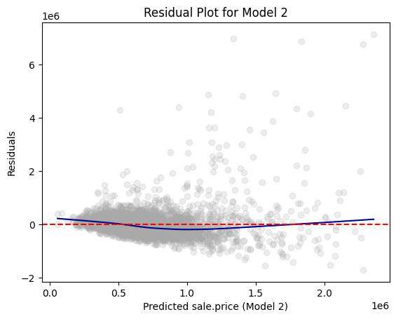
Residual Plots

• Residual plot is a scatterplot of fitted values and residuals.

  • A variable of fitted values on x-axis
  • A variable of residuals on y-axis

• A residual plot can be used to diagnose the quality of model results.

• Because we assume that \(\epsilon_{i}\) have a mean value of 0 with constant variance \(\sigma^2\), a well-behaved residual plot should bounce randomly and form a cloud roughly at the level of zero residual, the perfect prediction line.

• From the residual plot, we should ask the following the two questions ourselves:

  • On average, are the predictions correct?
  • Are there systematic errors?

Residual Plots

• On average, are the predictions correct?
• Are there systematic errors?

Residual Plots

Unbiasedness and Homoskedasticity

• We would like have a residual plot to be
  • Unbiased: have an average value of zero in any thin vertical strip;
  • Homoskedastic, which means “same stretch”: it is ideal to have the same spread of the residuals in any thin vertical strip.
  • When the variance of residuals changes across predicted values (e.g., residuals get larger as predicted values increase), the model suffers from heteroscedasticity.

Residual Plots

Examples

Residual Plots

What happens if biased?

• The model consistently overpredicts or underpredicts for certain values.
  • Indicates that the model might be misspecified—perhaps missing important variables or using an incorrect functional form.
  • Leads to biased parameter estimates, meaning the coefficients are systematically off, reducing the validity of predictions and inferences.

Residual Plots

What happens if heteroscedasticity is present?

• Consequences of heteroscedasticity:
  • 📉 Inefficient coefficient estimates: Estimates remain unbiased but are no longer efficient (i.e., they don’t have the smallest variance).
  • ❌ Biased standard errors: Leads to unreliable p-values and confidence intervals, potentially resulting in invalid hypothesis tests.
  • ⚠️ Misleading inferences: Predictors may appear statistically significant or insignificant incorrectly.
  • 🎯 Poor predictive performance: The model might perform poorly on future data, especially if the residual variance grows with higher predicted values.

Residual Plots in Python

• PySpark itself does not have built-in visualization capabilities.
  • Firstly, we convert PySpark DataFrame into Pandas DataFrame by using .toPandas()

# Residual plot for Model 2:
# Convert test predictions to Pandas
rdf = dtest2.select(["prediction", "sale_price"]).toPandas()
rdf["residual"] = rdf["sale_price"] - rdf["prediction"]

Residual Plots in Python

• We then use matplotlib.pyplot to draw a residual plot:

import matplotlib.pyplot as plt
import statsmodels.api as sm  # for lowess smoothing

plt.scatter(rdf["prediction"], rdf["residual"], alpha=0.2, color="darkgray")

# Use lowess smoothing for the trend line
smoothed = sm.nonparametric.lowess(rdf["residual"], rdf["prediction"])
plt.plot(smoothed[:, 0], smoothed[:, 1], color="darkblue")

# Perfect prediction line
#   A horizontal line at residual = 0
plt.axhline(y=0, color="red", linestyle="--")

# Labeling
plt.xlabel("Predicted sale.price (Model 2)")
plt.ylabel("Residuals")
plt.title("Residual Plot for Model 2")
plt.show()

Hypothesis Testing on Beta Coefficient

Hypothesis Testing on Beta Coefficient

• To determine whether an independent variable has a statistically significant effect on the dependent variable in a linear regression model.

• Consider the following linear regression model: \[ y_{i} = \beta_0 + \beta_1 x_{1,i} + \beta_2 x_{2,i} + \dots + \beta_k x_{k,i} + \epsilon_{i} \]

• \(y\): Outcome

• \(x_1, x_2, \dots, x_k\): Predictors

• \(\beta_0\): Intercept
  

• \(\beta_1, \beta_2, \dots, \beta_k\): Coefficients
  

• \(\epsilon_{i}\): Error term

Hypotheses and Test Statistic

• We test whether a specific coefficient \(\beta_j\) significantly differs from zero:
  • Null Hypothesis (\(H_0\)): \(\beta_j = 0\) (No relationship)
    
  • Alternative Hypothesis (\(H_A\)): \(\beta_j \neq 0\) (Significant relationship)
• The t-statistic is used to test each coefficient:

\[ t = \frac{\hat{\beta_j} - 0}{SE(\hat{\beta_j})} \]

• \(\hat{\beta_j}\): Estimated coefficient
  
• \(SE(\hat{\beta_j})\): Standard error of the estimate

Hypothesis Testing - Decision Rule and Interpretation

1. Calculate the p-value based on the t-distribution with \(n - k - 1\) degrees of freedom.
2. Compare p-value with significance level \(\alpha\) (e.g., 0.05):
   • If \(p \leq \alpha\): Reject \(H_0\) (Significant)
   • If \(p > \alpha\): Fail to reject \(H_0\) (Not significant)

• In our course, stars in a regression table mean a significance level:
  • * (10%); ** (5%); *** (1%)
• Reject \(H_0\): There is sufficient evidence to suggest a statistically significant relationship between \(x_j\) and \(y\).
• Fail to reject \(H_0\): No statistically significant evidence of a relationship between \(x_j\) and \(y\).

Interpreting Beta Estimates

Interpreting Estimated Beta Coefficients

Example

The model equation is \[\begin{align} \texttt{sale_price[i]} \;=\;\, &\texttt{b0} \,+\,\\ &\texttt{b1*gross_square_feet[i]} \,+\,\texttt{b2*age[i]}\,+\,\\ &\texttt{b3*Bronx[i]} \,+\,\texttt{b4*Brooklyn[i]} \,+\,\\&\texttt{b5*Queens[i]} \,+\,\texttt{b6*Staten Island[i]}\,+\,\\ &\texttt{e[i]} \end{align}\] - The reference level of borough_name variables is Manhattan.

Interpreting Estimated Beta Coefficients

1. gross_square_feet

• Consider the predicted sales prices of the two houses, A and B.
  • Both A and B are in Bronx and with the same age.
  • gross_square_feet of house A is 2001, while that of house B is 2000.
• All else being equal, an increase in gross_square_feet by one unit is associated with an increase in sale_price by \(\hat{\beta_{1}}\).
  • Why?

Interpreting Estimated Beta Coefficients

1. gross_square_feet

\[ \begin{align}\widehat{\texttt{sale_price[A]}} \;=\quad& \hat{\texttt{b0}} \,+\, \hat{\texttt{b1}}\texttt{*gross_square_feet[A]} \,+\, \hat{\texttt{b2}}\texttt{*age[A]} \,+\,\\ &\hat{\texttt{b3}}\texttt{*Bronx[A]}\,+\,\hat{\texttt{b4}}\texttt{*Brooklyn[A]} \,+\,\\ &\hat{\texttt{b5}}\texttt{*Queens[A]}\,+\, \hat{\texttt{b6}}\texttt{*Staten Island[A]}\\ \widehat{\texttt{sale_price[B]}} \;=\quad& \hat{\texttt{b0}} \,+\, \hat{\texttt{b1}}\texttt{*gross_square_feet[B]} \,+\, \hat{\texttt{b2}}\texttt{*age[B]}\,+\,\\ &\hat{\texttt{b3}}\texttt{*Bronx[B]}\,+\, \hat{\texttt{b4}}\texttt{*Brooklyn[B]} \,+\,\\ &\hat{\texttt{b5}}\texttt{*Queens[B]}\,+\, \hat{\texttt{b6}}\texttt{*Staten Island[B]} \end{align} \]

\[ \begin{align}\Leftrightarrow\qquad&\widehat{\texttt{sale_price[A]}} \,-\, \widehat{\texttt{sale_price[B]}}\qquad \\ \;=\quad &\hat{\texttt{b1}}\texttt{*}(\texttt{gross_square_feet[A]} - \texttt{gross_square_feet[B]})\\ \;=\quad &\hat{\texttt{b1}}\texttt{*}\texttt{(2001 - 2000)} \,=\, \hat{\texttt{b1}}\qquad\qquad\quad\;\; \end{align} \]

Interpreting Estimated Beta Coefficients

2. borough_nameBronx

• Consider the predicted sales prices of the two houses, A and C.

  • Both A and C are with the same age and the same gross_square_feet.
  • A is in Bronx, and C is in Manhattan.

• All else being equal, an increase in borough_nameBronx by one unit is associated with an increase in sale_price by b3.

• Equivalently, all else being equal, being in Bronx relative to being a in Manhattan is associated with a decrease in sale_price by |b3|.

  • Why?

Interpreting Estimated Beta Coefficients

2. borough_nameBronx

\[ \begin{align}\widehat{\texttt{sale_price[A]}} \;=\quad& \hat{\texttt{b0}} \,+\, \hat{\texttt{b1}}\texttt{*gross_square_feet[A]} \,+\, \hat{\texttt{b2}}\texttt{*age[A]} \,+\,\\ &\hat{\texttt{b3}}\texttt{*Bronx[A]}\,+\, \hat{\texttt{b4}}\texttt{*Brooklyn[A]} \,+\,\\ &\hat{\texttt{b5}}\texttt{*Queens[A]}\,+\, \hat{\texttt{b6}}\texttt{*Staten Island[A]}\\ \widehat{\texttt{sale_price[C]}} \;=\quad& \hat{\texttt{b0}} \,+\, \hat{\texttt{b1}}\texttt{*gross_square_feet[C]} \,+\, \hat{\texttt{b2}}\texttt{*age[C]}\,+\,\\ &\hat{\texttt{b3}}\texttt{*Bronx[C]}\,+\, \hat{\texttt{b4}}\texttt{*Brooklyn[C]} \,+\,\\ &\hat{\texttt{b5}}\texttt{*Queens[C]}\,+\, \hat{\texttt{b6}}\texttt{*Staten Island[C]} \end{align} \]

\[ \begin{align}\Leftrightarrow\qquad&\widehat{\texttt{sale_price[A]}} \,-\, \widehat{\texttt{sale_price[C]}}\qquad \\ \;=\quad &\hat{\texttt{b3}}\texttt{*}\texttt{Bronx[A]} \\ \;=\quad &\hat{\texttt{b3}}\qquad\qquad\qquad\qquad\quad\;\;\;\,\end{align} \]

Coefficient Plots in Python

• A coefficient plot shows beta estimates and their confidence intervals.

import matplotlib.pyplot as plt
import pandas as pd

# Create a Pandas DataFrame from model3's summary information
terms = assembler3.getInputCols()
coefs = model3.coefficients.toArray()[:len(terms)]
stdErrs = model3.summary.coefficientStandardErrors[:len(terms)]

df_summary = pd.DataFrame({
    "term": terms,
    "estimate": coefs,
    "std_error": stdErrs
})

# Plot using the DataFrame columns
plt.errorbar(df_summary["term"], df_summary["estimate"],
             yerr = 1.96 * df_summary["std_error"], fmt='o', capsize=5)
plt.xlabel("Terms")
plt.ylabel("Coefficient Estimate")
plt.title("Coefficient Estimates (Model 2)")
plt.axhline(0, color="red", linestyle="--")  # Add horizontal line at 0
plt.xticks(rotation=45)
plt.show()

Linear Regression with Log Transformation

Linear Regression with Log Transformation

The model equation with log-transformed \(\texttt{sale.price[i]}\) is \[\begin{align} \log(\texttt{sale.price[i]}) \;=\;\, &\texttt{b0} \,+\,\\ &\texttt{b1*gross.square.feet[i]} \,+\,\texttt{b2*age[i]}\,+\,\\ &\texttt{b3*Bronx[i]} \,+\,\texttt{b4*Brooklyn[i]} \,+\,\\&\texttt{b5*Queens[i]} \,+\,\texttt{b6*Staten Island[i]}\,+\,\\ &\texttt{e[i]}. \end{align}\]

• Note that the reference level for borough_name is Manhattan.

Beta Estimates for Log-transformed Variables

1. gross_square_feet

• Let’s re-consider the two properties \(\texttt{A}\) and \(\texttt{B}\).
  • \(\texttt{gross.square.feet[A]} = 2001\) and \(\texttt{gross.square.feet[B]} = 2000\).
  • Both are in the same borough.
  • Both properties’ ages are the same.

Beta Estimates for Log-transformed Variables

1. gross_square_feet

• If we apply the rule above for \(\widehat{\texttt{sale.price}}\texttt{[A]}\) and \(\widehat{\texttt{sale.price}}\texttt{[B]}\),

\[\begin{align}&\log(\widehat{\texttt{sale.price}}\texttt{[A]}) - \log(\widehat{\texttt{sale.price}}\texttt{[B]}) \\ \,=\, &\hat{\texttt{b1}}\,*\,(\texttt{gross.square.feet[A]} \,-\, \texttt{gross.square.feet[B]})\\ \,=\, &\hat{\texttt{b1}}\end{align}\]

So we can have the following: \[ \begin{align} &\Leftrightarrow\qquad\frac{\widehat{\texttt{sale.price[A]}}}{ \widehat{\texttt{sale.price[B]}}} \;=\; \texttt{exp(}\hat{\texttt{b1}}\texttt{)}\\ \quad&\Leftrightarrow\qquad\widehat{\texttt{sale.price[A]}} \;=\; \widehat{\texttt{sale.price[B]}} * \texttt{exp(}\hat{\texttt{b1}}\texttt{)} \end{align} \]

Beta Estimates for Log-transformed Variables

1. gross_square_feet

• Suppose \(\texttt{exp(}\hat{\texttt{b2}}\texttt{)} = 1.000431\).
  • Then \(\widehat{\texttt{sale.price[A]}}\) is \(1.000431\times\widehat{\texttt{sale.price[B]}}\).
  • All else being equal, an increase in \(\texttt{gross.square.feet}\) by one unit is associated with an increase in \(\texttt{sale.price}\) by 0.0431%.

Beta Estimates for Log-transformed Variables

2. borough_nameBronx

• Let’s re-consider the two properties \(\texttt{A}\) and \(\texttt{C}\).
  • A is in Bronx, and C is in Manhattan.
  • Both A and C’s age are the same.
  • Both A and C’s gross.square.feet are the same.

Beta Estimates for Log-transformed Variables

2. borough_nameBronx

• If we apply the log()-exp() rules for \(\widehat{\texttt{sale.price}}\texttt{[A]}\) and \(\widehat{\texttt{sale.price}}\texttt{[C]}\),

\[\begin{align}&\log(\widehat{\texttt{sale.price}}\texttt{[A]}) - \log(\widehat{\texttt{sale.price}}\texttt{[C]}) \\ \,=\, &\hat{\texttt{b3}}\,*\,(\texttt{borough_Bronx[A]} \,-\, \texttt{borough_Bronx[C]})\,=\, \hat{\texttt{b3}}\end{align}\]

So we can have the following: \[ \begin{align}&\Leftrightarrow\qquad\frac{\widehat{\texttt{sale.price[A]}}}{ \widehat{\texttt{sale.price[C]}}} \;=\; \texttt{exp(}\hat{\texttt{b3}}\texttt{)}\\ \quad&\Leftrightarrow\qquad\,\widehat{\texttt{sale.price[A]}} \;=\; \widehat{\texttt{sale.price[C]}} * \texttt{exp(}\hat{\texttt{b3}}\texttt{)} \end{align} \]

Beta Estimates for Log-transformed Variables

2. borough_nameBronx

• Suppose \(\texttt{exp(}\hat{\texttt{b3}}\texttt{)} = 0.2831691\).
  • Then \(\widehat{\texttt{sale.price[A]}}\) is \(0.2831691\times\widehat{\texttt{sale.price[B]}}\).
  • All else being equal, an increase in \(\texttt{borough_Bronx}\) by one unit is associated with a decrease in \(\texttt{sale.price}\) by (1 - 0.2831691) = 71.78%.
  • All else being equal, being in Bronx relative to being in Manhattan is associated with a decrease in \(\texttt{sale.price}\) by 71.78%.

Log-transformed Variables in PySpark

• We use the log() function to add a log-transformed variable:

from pyspark.sql.functions import log
sale_df = sale_df.withColumn("log_sale_price", 
                              log( sale_df['sale_price'] ) ) 

• To use a exponential function, we can use an exp() function from numpy:

import numpy as np

np.exp(1)
np.exp([1, 2, 3])

Linear Regression with Interaction Terms

Linear Regression with Interaction Terms

Motivation

• Does the relationship between sale.price and gross.square.feet vary by borough_name?

  • How can linear regression address the question above?

Linear Regression with Interaction Terms

Model

• The linear regression with an interaction between predictors \(X_{1}\) and \(X_{2}\) are:

\[Y_{\texttt{i}} \,=\, b_{0} \,+\, b_{1}\,X_{1,\texttt{i}} \,+\, b_{2}\,X_{2,\texttt{i}} \,+\, b_{3}\,X_{1,\texttt{i}}\times \color{Red}{X_{2,\texttt{i}}} \,+\, e_{\texttt{i}},\]

• where
  • \(i\;\): \(\;\;i\)-th observation in the training DataFrame, \(i = 1, 2, 3, \cdots\).
  • \(Y_{i}\,\): \(\;i\)-th observation of outcome \(Y\).
  • \(X_{p, i}\,\): \(i\)-th observation of the \(p\)-th predictor \(X_{p}\).
  • \(e_{i}\;\): \(\;i\)-th observation of statistical error.

Linear Regression with Interaction Terms

Model

• The linear regression with an interaction between predictors \(X_{1}\) and \(X_{2}\) are:

\[Y_{\texttt{i}} \,=\, b_{0} \,+\, b_{1}\,X_{1,\texttt{i}} \,+\, b_{2}\,X_{2,\texttt{i}} \,+\, b_{3}\,X_{1,\texttt{i}}\times \color{Red}{X_{2,\texttt{i}}} \,+\, e_{\texttt{i}}\;.\]

Interaction

• The relationship between \(X_{1}\) and \(Y\) varies by values of \(b_{3}\, X_{2}\):

\[\frac{\Delta Y}{\Delta X_{1}} \,=\, b_{1} + b_{3}\, X_{2}\].

Example

• \(X_{2}\) is often a dummy variable. If \(b_{3} \neq 0\) and \(X_{2, \texttt{i}} = 1\),

\[\frac{\Delta Y}{\Delta X_{1}} \,=\, b_{1} + b_{3}\].

Linear Regression with Interaction Terms

Interaction with a Dummy Variable

• The linear regression with an interaction between predictors \(X_{1}\) and \(X_{2}\in\{\,0, 1\,\}\) are:

\[Y_{\texttt{i}} \,=\, b_{0} \,+\, b_{1}\,X_{1,\texttt{i}} \,+\, b_{2}\,X_{2,\texttt{i}} \,+\, b_{3}\,X_{1,\texttt{i}}\times \color{Red}{X_{2,\texttt{i}}} \,+\, e_{\texttt{i}},\] where \(X_{\,2, \texttt{i}}\) is either 0 or 1.

• For \(\texttt{i}\) such that \(X_{\,2, \texttt{i}} = 0\), the model is \[Y_{\texttt{i}} \,=\, b_{0} \,+\, b_{1}\,X_{1,\texttt{i}} \,+\, e_{\texttt{i}}\qquad\qquad\qquad\qquad\qquad\quad\;\;\]

• For \(\texttt{i}\) such that \(X_{\,2, \texttt{i}} = 1\), the model is

\[Y_{\texttt{i}} \,=\, (\,b_{0} \,+\, b_{2}\,) \,+\, (\,b_{1}\,+\, b_{3}\,)\,X_{1,\texttt{i}} \,+\, e_{\texttt{i}}\qquad\qquad\]

Linear Regression with Interaction Terms

Motivation

• Is sale.price related with gross.square.feet?

\[ \begin{align} \texttt{sale_price[i]} \;=\;\, &\texttt{b0} \,+\,\\ &\texttt{b1*Bronx[i]} \,+\,\texttt{b2*Brooklyn[i]} \,+\,\\&\texttt{b3*Queens[i]} \,+\,\texttt{b4*Staten Island[i]}\,+\,\\ &\texttt{b5*age[i]}\,+\,\\ &\texttt{b6*gross_square_feet[i]} \,+\,\texttt{e[i]} \end{align} \]

Linear Regression with Interaction Terms

Motivation

• Does the relationship between sale.price and gross.square.feet vary by borough_name?

\[ \begin{align} \texttt{sale_price[i]} \;=\;\, &\texttt{b0} \,+\,\\ &\texttt{b1*Bronx[i]} \,+\,\texttt{b2*Brooklyn[i]} \,+\,\\ &\texttt{b3*Queens[i]} \,+\,\texttt{b4*Staten Island[i]}\,+\, \\ &\texttt{b5*age[i]}\,+\,\\ &\texttt{b6*gross_square_feet[i]} \,+\,\\ &\texttt{b7*gross_square_feet[i]*Bronx[i]} \,+\, \\ &\texttt{b8*gross_square_feet[i]*Brooklyn[i]} \,+\, \\ &\texttt{b9*gross_square_feet[i]*Queens[i]} \,+\, \\ &\texttt{b10*gross_square_feet[i]*Staten Island[i]} \,+\, \texttt{e[i]} \\ \end{align} \]

Log-Log Linear Regression

Log-Log Linear Regression

• To estimate the price elasticity of orange juice (OJ), we will use sales data for OJ from Dominick’s grocery stores in the 1990s.
  • Weekly price and sales (in number of cartons “sold”) for three OJ brandsTropicana, Minute Maid, Dominick’s
  • A dummy, ad, showing whether each brand was advertised (in store or flyer) that week.

Variable	Description
sales	Quantity of OJ cartons sold
price	Price of OJ
brand	Brand of OJ
ad	Advertisement status

Log-Log Linear Regression

Estimating Price Elasticity

• Let’s prepare the OJ data:

oj = pd.read_csv('https://bcdanl.github.io/data/dominick_oj_feat.csv')

Log-Log Linear Regression

Estimating Price Elasticity

• The following model estimates the price elasticity of demand for a carton of OJ:

\[\begin{align} \log(\texttt{sales}_{\texttt{i}}) &\,=\, \;\; b_{\texttt{intercept}} \,+\, b_{\,\texttt{mm}}\,\texttt{brand}_{\,\texttt{mm}, \texttt{i}} \,+\, b_{\,\texttt{tr}}\,\texttt{brand}_{\,\texttt{tr}, \texttt{i}}\\ &\quad\,+\, b_{\texttt{price}}\,\log(\texttt{price}_{\texttt{i}}) \,+\, e_{\texttt{i}},\\ \text{where}\qquad\qquad&\\ \texttt{brand}_{\,\texttt{tr}, \texttt{i}} &\,=\, \begin{cases} \texttt{1} & \text{ if an orange juice } \texttt{i} \text{ is } \texttt{Tropicana};\\\\ \texttt{0} & \text{otherwise}.\qquad\qquad\quad\, \end{cases}\\ \texttt{brand}_{\,\texttt{mm}, \texttt{i}} &\,=\, \begin{cases} \texttt{1} & \text{ if an orange juice } \texttt{i} \text{ is } \texttt{Minute Maid};\\\\ \texttt{0} & \text{otherwise}.\qquad\qquad\quad\, \end{cases} \end{align}\]

Log-Log Linear Regression

Estimating Price Elasticity

• The following model estimates the price elasticity of demand for a carton of OJ:

\[\log(\texttt{sales}_{\texttt{i}}) \,=\, \quad\;\; b_{\texttt{intercept}} \,+\, b_{\,\texttt{mm}}\,\texttt{brand}_{\,\texttt{mm}, \texttt{i}} \,+\, b_{\,\texttt{tr}}\,\texttt{brand}_{\,\texttt{tr}, \texttt{i}}\\ \,+\, b_{\texttt{price}}\,\log(\texttt{price}_{\texttt{i}}) \,+\, e_{\texttt{i}}\]

• When \(\texttt{brand}_{\,\texttt{tr}, \texttt{i}}\,=\,0\) and \(\texttt{brand}_{\,\texttt{mm}, \texttt{i}}\,=\,0\), the beta coefficient for the intercept \(b_{\texttt{intercept}}\) gives the value of Dominick’s log sales at \(\log(\,\texttt{price[i]}\,) = 0\).

• The beta coefficient \(b_{\texttt{price}}\) is the price elasticity of demand.

  • It measures how sensitive the quantity demanded is to its price.

Log-Log Linear Regression

Estimating Price Elasticity

• For small changes in variable \(x\) from \(x_{0}\) to \(x_{1}\), the following equation holds:

\[\Delta \log(x) \,= \, \log(x_{1}) \,-\, \log(x_{0}) \approx\, \frac{x_{1} \,-\, x_{0}}{x_{0}} \,=\, \frac{\Delta\, x}{x_{0}}.\]

• The coefficient on \(\log(\texttt{price}_{\texttt{i}})\), \(b_{\texttt{price}}\), is therefore

\[b_{\texttt{price}} \,=\, \frac{\Delta \log(\texttt{sales}_{\texttt{i}})}{\Delta \log(\texttt{price}_{\texttt{i}})}\,=\, \frac{\frac{\Delta \texttt{sales}_{\texttt{i}}}{\texttt{sales}_{\texttt{i}}}}{\frac{\Delta \texttt{price}_{\texttt{i}}}{\texttt{price}_{\texttt{i}}}}.\]

• All else being equal, an increase in \(\texttt{price}\) by 1% is associated with a decrease in \(\texttt{sales}\) by \(b_{\texttt{price}}\)%.

Log-Log Linear Regression

EDA

• Describe the relationship between log(price) and log(sales) by brand.

import pandas as pd
import numpy as np
import seaborn as sns
import matplotlib.pyplot as plt

oj['log_price'] = oj['price'].apply(lambda x: np.log(x))
oj['log_sales'] = oj['sales'].apply(lambda x: np.log(x))

sns.lmplot(
    x='log_price', 
    y='log_sales', 
    hue='brand',     # color by brand
    data=oj, 
    aspect=1.2, 
    height=5,
    markers=["o", "s", "D"],  # optional: different markers per brand
    scatter_kws={'alpha': 0.025},  # Pass alpha to the scatter plot
    legend=True
)

Log-Log Linear Regression

EDA

• Describe the relationship between log(price) and log(sales) by brand and ad.

sns.lmplot(
    x='log_price', 
    y='log_sales', 
    hue='brand',     # color by brand
    col='ad',         # facet by feat
    data=oj, 
    aspect=1.2, 
    height=5,
    markers=["o", "s", "D"],  # optional: different markers per brand
    # Pass alpha to the scatter plot
    scatter_kws={'alpha': 0.025},
    col_wrap=2,         # how many facets per row
    legend=True
)

Log-Log Linear Regression

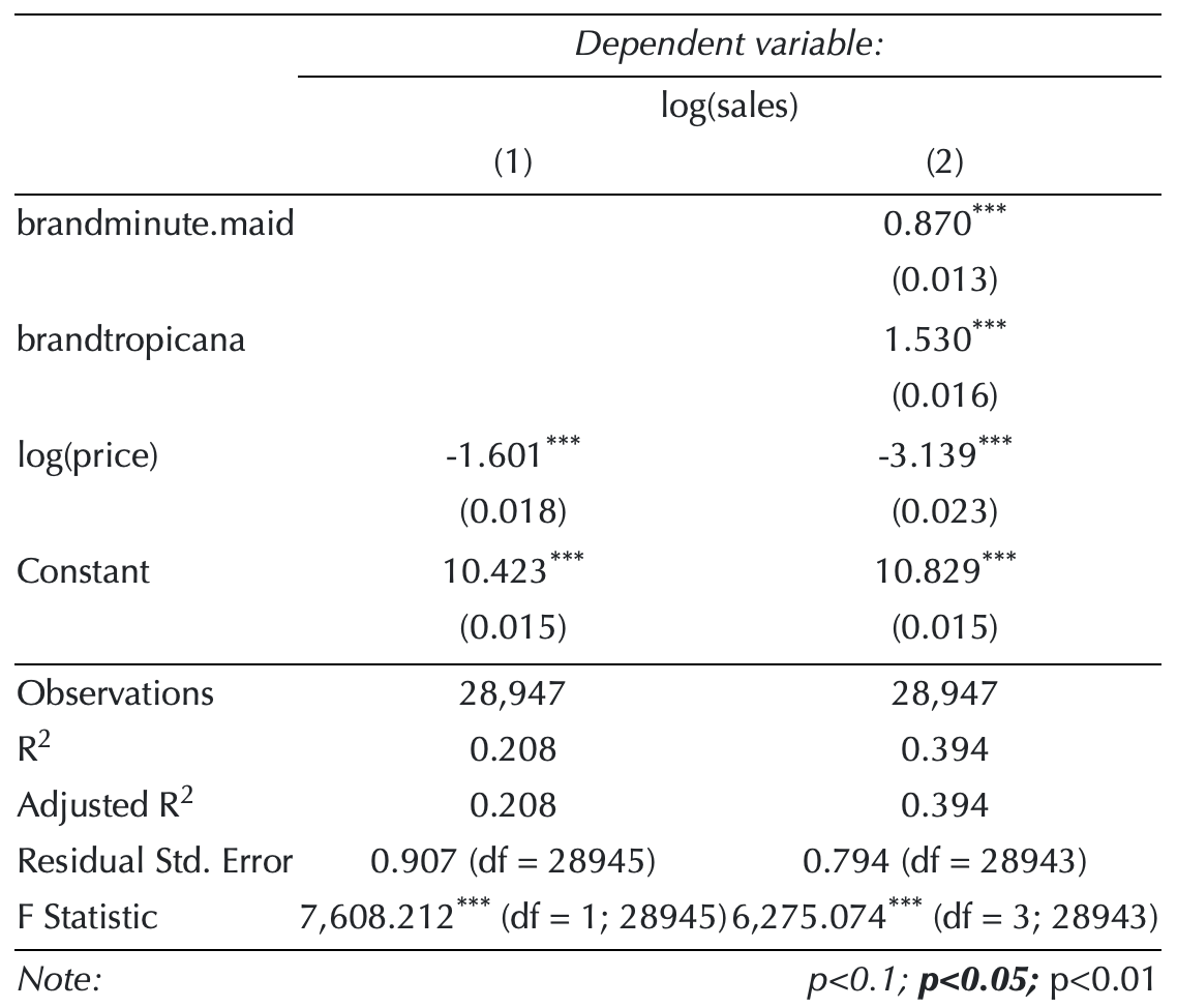
Estimating Price Elasticity

• Let’s train the first model, model_1:

\[ \begin{align} \log(\texttt{sales}_{\texttt{i}}) \,=\, &\quad\;\; b_{\texttt{intercept}} \\ &\,+\,b_{\,\texttt{mm}}\,\texttt{brand}_{\,\texttt{mm}, \texttt{i}} \,+\, b_{\,\texttt{tr}}\,\texttt{brand}_{\,\texttt{tr}, \texttt{i}}\\ &\,+\, b_{\texttt{price}}\,\log(\texttt{price}_{\texttt{i}}) \,+\, e_{\texttt{i}} \end{align} \]

Log-Log Linear Regression

Estimating Price Elasticity

• How does the relationship between log(sales) and log(price) vary by brand?

  • Let’s train the second model, model_2, that addresses the above question:

\[ \begin{align} \log(\texttt{sales}_{\texttt{i}}) \,=\,&\;\; \quad b_{\texttt{intercept}} \,+\, \color{Green}{b_{\,\texttt{mm}}\,\texttt{brand}_{\,\texttt{mm}, \texttt{i}}} \,+\, \color{Blue}{b_{\,\texttt{tr}}\,\texttt{brand}_{\,\texttt{tr}, \texttt{i}}}\\ &\,+\, b_{\texttt{price}}\,\log(\texttt{price}_{\texttt{i}}) \\ &\, +\, b_{\texttt{price*mm}}\,\log(\texttt{price}_{\texttt{i}})\,\times\,\color{Green} {\texttt{brand}_{\,\texttt{mm}, \texttt{i}}} \\ &\,+\, b_{\texttt{price*tr}}\,\log(\texttt{price}_{\texttt{i}})\,\times\,\color{Blue} {\texttt{brand}_{\,\texttt{tr}, \texttt{i}}} \,+\, e_{\texttt{i}} \end{align} \]

Log-Log Linear Regression

• For \(\texttt{i}\) such that \(\color{Green}{\texttt{brand}_{\,\texttt{mm}, \texttt{i}}} = 0\) and \(\color{Blue}{\texttt{brand}_{\,\texttt{tr}, \texttt{i}}} = 0\), the model equation is: \[\log(\texttt{sales}_{\texttt{i}}) \,=\, \; \,b_{\texttt{intercept}}\qquad\qquad\qquad\qquad\qquad\qquad\qquad\qquad\\ \qquad\,+\, b_{\texttt{price}} \,\log(\texttt{price}_{\texttt{i}}) \,+\, e_{\texttt{i}}\,.\qquad\qquad\;\]

• For \(\texttt{i}\) such that \(\color{Green}{\texttt{brand}_{\,\texttt{mm}, \texttt{i}}} = 1\) and \(\color{Blue}{\texttt{brand}_{\,\texttt{tr}, \texttt{i}}} = 0\), the model equation is: \[\log(\texttt{sales}_{\texttt{i}}) \,=\, \; (\,b_{\texttt{intercept}} \,+\, b_{\,\texttt{mm}}\,)\qquad\qquad\qquad\qquad\qquad\qquad\qquad\\ \qquad\!\,+\,(\, b_{\texttt{price}} \,+\, \color{Green}{b_{\texttt{price*mm}}}\,)\,\log(\texttt{price}_{\texttt{i}}) \,+\, e_{\texttt{i}}\,.\]

• For \(\texttt{i}\) such that \(\color{Green}{\texttt{brand}_{\,\texttt{mm}, \texttt{i}}} = 0\) and \(\color{Blue}{\texttt{brand}_{\,\texttt{tr}, \texttt{i}}} = 1\), the model equation is: \[\log(\texttt{sales}_{\texttt{i}}) \,=\, \; (\,b_{\texttt{intercept}} \,+\, b_{\,\texttt{tr}}\,)\qquad\qquad\qquad\qquad\qquad\qquad\qquad\\ \qquad\!\,+\,(\, b_{\texttt{price}} \,+\, \color{Blue}{b_{\texttt{price*tr}}}\,)\,\log(\texttt{price}_{\texttt{i}}) \,+\, e_{\texttt{i}}\,.\]

Adding Interaction Terms in PySpark

• The UDF add_interaction_terms requires at least two lists of variable names.

• var_list3 is optional.

  • If var_list3 is provided, the add_interaction_terms function adds all possible two-way interactions and three-way interaction to the dtrain and dtest DataFrames.

def add_interaction_terms(var_list1, var_list2, var_list3=None):
    """
    Creates interaction term columns in the global DataFrames dtrain and dtest.

    For two sets of variable names (which may represent categorical (dummy) or continuous variables),
    this function creates two-way interactions by multiplying each variable in var_list1 with each
    variable in var_list2.

    Optionally, if a third list of variable names (var_list3) is provided, the function also creates
    three-way interactions among each variable in var_list1, each variable in var_list2, and each variable
    in var_list3.

    Parameters:
        var_list1 (list): List of column names for the first set of variables.
        var_list2 (list): List of column names for the second set of variables.
        var_list3 (list, optional): List of column names for the third set of variables for three-way interactions.

    Returns:
        A flat list of new interaction column names.
    """
    global dtrain, dtest

    interaction_cols = []

    # Create two-way interactions between var_list1 and var_list2.
    for var1 in var_list1:
        for var2 in var_list2:
            col_name = f"{var1}_*_{var2}"
            dtrain = dtrain.withColumn(col_name, col(var1).cast("double") * col(var2).cast("double"))
            dtest = dtest.withColumn(col_name, col(var1).cast("double") * col(var2).cast("double"))
            interaction_cols.append(col_name)

    # Create two-way interactions between var_list1 and var_list3.
    if var_list3 is not None:
      for var1 in var_list1:
          for var3 in var_list3:
              col_name = f"{var1}_*_{var3}"
              dtrain = dtrain.withColumn(col_name, col(var1).cast("double") * col(var3).cast("double"))
              dtest = dtest.withColumn(col_name, col(var1).cast("double") * col(var3).cast("double"))
              interaction_cols.append(col_name)

    # Create two-way interactions between var_list2 and var_list3.
    if var_list3 is not None:
      for var2 in var_list2:
          for var3 in var_list3:
              col_name = f"{var2}_*_{var3}"
              dtrain = dtrain.withColumn(col_name, col(var2).cast("double") * col(var3).cast("double"))
              dtest = dtest.withColumn(col_name, col(var2).cast("double") * col(var3).cast("double"))
              interaction_cols.append(col_name)

    # If a third list is provided, create three-way interactions.
    if var_list3 is not None:
        for var1 in var_list1:
            for var2 in var_list2:
                for var3 in var_list3:
                    col_name = f"{var1}_*_{var2}_*_{var3}"
                    dtrain = dtrain.withColumn(col_name, col(var1).cast("double") * col(var2).cast("double") * col(var3).cast("double"))
                    dtest = dtest.withColumn(col_name, col(var1).cast("double") * col(var2).cast("double") * col(var3).cast("double"))
                    interaction_cols.append(col_name)

    return interaction_cols

 # Example
 # interaction_cols_brand_price = add_interaction_terms(dummy_cols_brand, ['log_price'])
 # interaction_cols_brand_ad_price = add_interaction_terms(dummy_cols_brand, dummy_cols_ad, ['log_price'])

Log-Log Linear Regression

• How does advertisement play a role in the relationship between sales and prices in the OJ market?
  • The ads can increase sales at all prices.
  • They can change price sensitivity.
  • They can do both of these things in a brand-specific manner.
• What would be the formula that address the question above?

Log-Log Linear Regression

• Let’s train the third model, model_3, that addresses the question in the previous page:

\[ \begin{align} \log(\texttt{sales}_{\texttt{i}}) \,=\,\quad\;\;& b_{\texttt{intercept}} \,+\, \color{Green}{b_{\,\texttt{mm}}\,\texttt{brand}_{\,\texttt{mm}, \texttt{i}}} \,+\, \color{Blue}{b_{\,\texttt{tr}}\,\texttt{brand}_{\,\texttt{tr}, \texttt{i}}} \\ &\,+\; b_{\,\texttt{ad}}\,\color{Orange}{\texttt{ad}_{\,\texttt{i}}} \qquad\qquad\qquad\qquad\quad \\ &\,+\, b_{\texttt{mm*ad}}\,\color{Green} {\texttt{brand}_{\,\texttt{mm}, \texttt{i}}}\,\times\, \color{Orange}{\texttt{ad}_{\,\texttt{i}}}\,+\, b_{\texttt{tr*ad}}\,\color{Blue} {\texttt{brand}_{\,\texttt{tr}, \texttt{i}}}\,\times\, \color{Orange}{\texttt{ad}_{\,\texttt{i}}} \\ &\,+\; b_{\texttt{price}}\,\log(\texttt{price}_{\texttt{i}}) \qquad\qquad\qquad\;\;\;\;\, \\ &\,+\, b_{\texttt{price*mm}}\,\log(\texttt{price}_{\texttt{i}})\,\times\,\color{Green} {\texttt{brand}_{\,\texttt{mm}, \texttt{i}}}\qquad\qquad\qquad\;\, \\ &\,+\, b_{\texttt{price*tr}}\,\log(\texttt{price}_{\texttt{i}})\,\times\,\color{Blue} {\texttt{brand}_{\,\texttt{tr}, \texttt{i}}}\qquad\qquad\qquad\;\, \\ & \,+\, b_{\texttt{price*ad}}\,\log(\texttt{price}_{\texttt{i}})\,\times\,\color{Orange}{\texttt{ad}_{\,\texttt{i}}}\qquad\qquad\qquad\;\;\, \\ &\,+\, b_{\texttt{price*mm*ad}}\,\log(\texttt{price}_{\texttt{i}}) \,\times\,\,\color{Green} {\texttt{brand}_{\,\texttt{mm}, \texttt{i}}}\,\times\, \color{Orange}{\texttt{ad}_{\,\texttt{i}}} \\ &\,+\, b_{\texttt{price*tr*ad}}\,\log(\texttt{price}_{\texttt{i}}) \,\times\,\,\color{Blue} {\texttt{brand}_{\,\texttt{tr}, \texttt{i}}}\,\times\, \color{Orange}{\texttt{ad}_{\,\texttt{i}}} \,+\, e_{\texttt{i}} \end{align} \]

Log-Log Linear Regression

Estimating Price Elasticity

• Describe the relationship between ad and brand using stacked bar charts.

sns.histplot(
    data=oj,
    x='ad_status',   # categorical variable on the x-axis
    hue='brand',     # fill color by brand
    multiple='fill'  # 100% stacked bars
)
plt.ylabel('Proportion')

• Model 3 assumes that the relationship between price and sales can vary by ad.

Log-Log Linear Regression

Estimating Price Elasticity

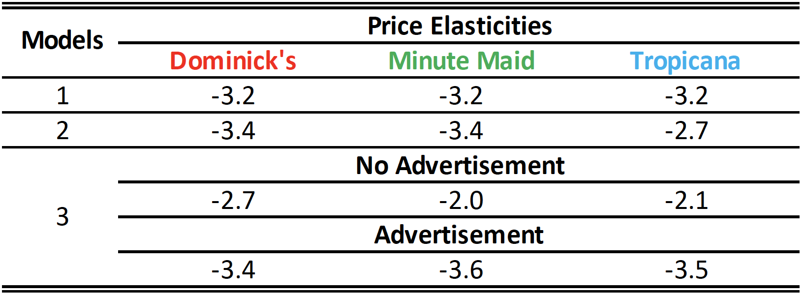
• How would you explain different estimation results across different models?

• Which model do you prefer? Why?