Lecture 6

Tree-based Model II: Ensemble Models

Byeong-Hak Choe

bchoe@geneseo.edu

SUNY Geneseo

March 30, 2026

🌲 Random Forest

Limitation of CART

• CART automatically learns non-linear response functions and will discover interactions between variables.
• Unfortunately, it is tough to avoid overfit with CART.
  • A single deep tree memorizes the training data rather than learning the true underlying pattern.
• Real structure of the tree is not easily chosen via cross validation.
• One way to mitigate the shortcomings of CART is bootstrap aggregation, or bagging.

Analogy: The Overconfident Student

• Think of a single CART tree like a student who memorizes every detail from last year’s exam. They ace that exam perfectly, but fail the new one because they memorized noise, not concepts.
• An ensemble model is like asking many students who studied different subsets of material, then taking their majority answer. The quirks of any one student cancel out.

Bootstrap

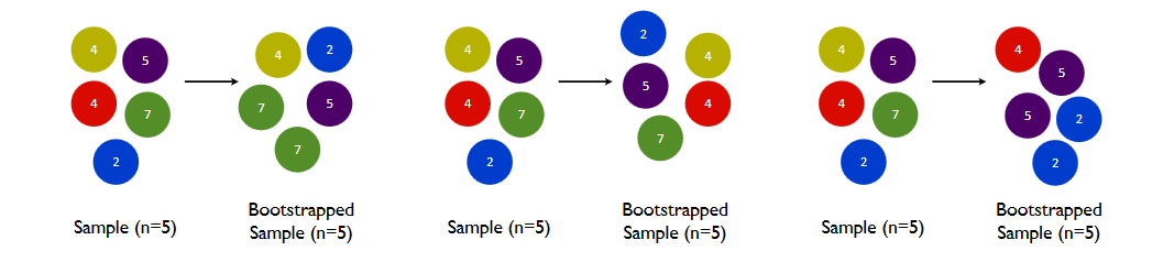
• Bootstrap is random sampling with replacement.
  • “With replacement” means the same observation can be drawn more than once into a single bootstrap sample.
  • On average, each bootstrap sample contains about 63% of the unique original observations — the rest are left out.
• Bootstrap is a reliable tool for uncertainty quantification.

Bagging (Bootstrap Aggregation)

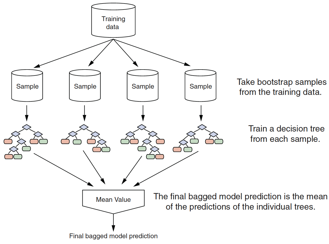
• Real structure that persists across datasets shows up in the average.
• A bagged ensemble of trees is also less likely to overfit the data.

Bagging: Reducing Variance by Averaging

• Step 1: Draw \(B\) bootstrap samples from the training data (random sampling with replacement)
• Step 2: Fit a full, deep decision tree on each bootstrap sample independently
• Step 3: Aggregate predictions:
  • Regression: average the \(B\) predictions
  • Classification: majority vote across the \(B\) trees
• Why does this work?
  • Each tree has high variance but is roughly unbiased
  • Averaging \(B\) independent unbiased estimates reduces variance by a factor of \(B\)
  • Real patterns that persist across bootstrap samples show up in the average; noise does not

Random Forest Algorithm

Random forests are an extension of bagging

• For each tree \(b\) in \(1, \dots, B\):
  • Construct a bootstrap sample from the training data
  • Grow a deep, unpruned, complicated (aka really overfit!) tree but with a twist
  • At each split: limit the variables considered to a random subset \(m_{try}\) of original \(p\) variables
• Predictions are made the same way as bagging:
  • Regression: take the average across the trees
  • Classification: take the majority vote across the trees
• Split-variable randomization adds more randomness to make each tree more independent of each other

Split-variable Randomization

• Random forest introduces \(m_{try}\) as a tuning parameter: typically use \(p / 3\) (regression) or \(\sqrt{p}\) (classification)
  • At each split, only a random subset of \(m_{try}\) predictors is considered — not all \(p\) predictors.
  • This forces trees to use different variables, so their errors do not all correlate with each other.
    • Smaller \(m_{try}\): More randomness → more diverse trees → potentially better generalization.
    • Larger \(m_{try}\): Less randomness → trees are more similar → can lead to overfitting/underfitting depending on data.
  • \(m_{try} = p\) is bagging (use all predictors at every split.)

Why Decorrelating Trees Helps

• Imagine you survey 500 friends, but they all watch the same news channel — their answers are all correlated.
• Averaging them barely reduces uncertainty.
• If each friend independently formed their opinion, the average is much more reliable.
• Random forest does the same: by limiting which predictors each tree can use at each split, trees become more independent, so averaging them is more powerful.

Random Forest Diagram

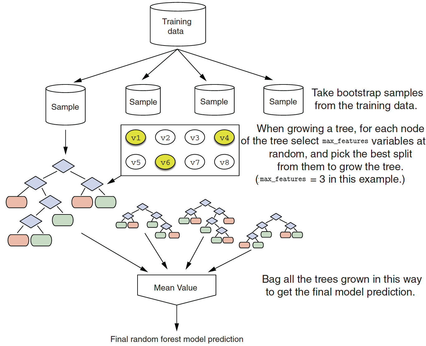
• The final ensemble of trees is bagged to make the random forest predictions.

Accuracy of the Tree

• For classification, accuracy = \(\frac{\text{Number of Correct Prediction}}{\text{Total Prediction}}\).

• For regression, accuracy means \(R^{2}\).

  • \(R^2 = 1\): model explains all variability
  • \(R^2 = 0\): model explains none of it

Out-of-bag Samples for Estimating the Accuracy

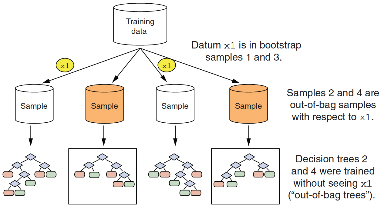
Out-of-bag samples for observation x1

• Since random forest uses a large number of bootstrap samples, each data point has a corresponding set of out-of-bag samples.

OOB Error: Free Cross-Validation

• For each observation \(x_i\), only the trees that were not trained on it (its out-of-bag trees) are used to generate a prediction.
• Aggregating these OOB predictions across all observations gives the OOB error — a nearly unbiased estimate of test error, with no need for a separate validation set.
• This makes random forest computationally efficient: training and evaluation happen in one pass.

Examining Variable Importance

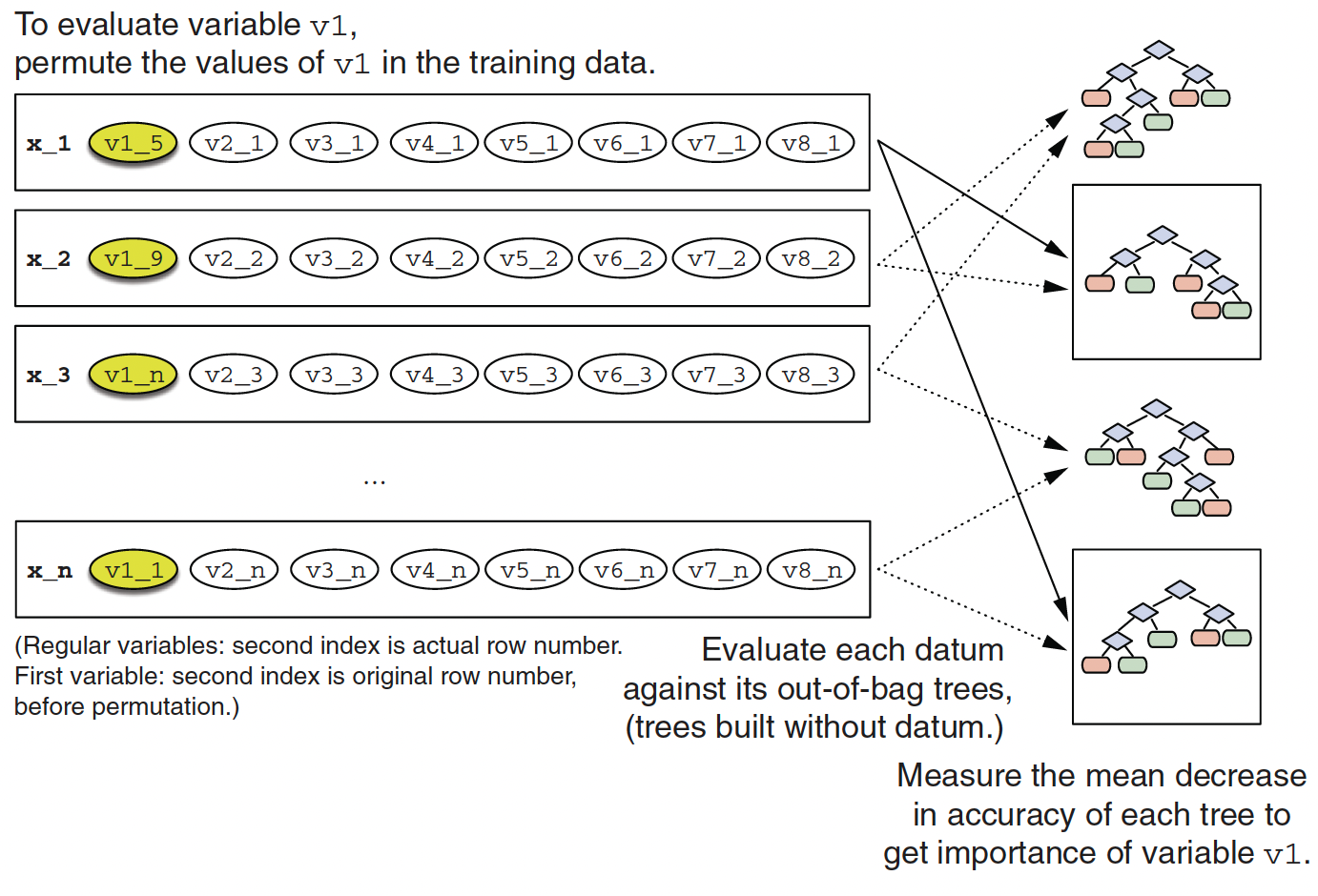
Calculating variable importance of variable v1

VIP: Why Shuffle Instead of Remove?

• To measure how important variable \(v_1\) is: randomly shuffle \(v_1\)’s values across all observations, then re-evaluate each out-of-bag tree.
• If accuracy drops a lot after shuffling, \(v_1\) is highly important — the model was relying on it.
• If accuracy barely changes, \(v_1\) carries little predictive signal.

Note

Removing a variable entirely changes the model. Shuffling breaks the relationship between \(v_1\) and the outcome while keeping the variable present — a controlled experiment that isolates each variable’s contribution.

🚀 Gradient-boosted Trees

Gradient-boosted Trees

• Gradient boosting tries to improve prediction performance by sequentially adding trees to an existing ensemble:

1. Use the current ensemble \(TE\) to make predictions on the training data.
2. Measure the residuals between the true outcomes and the predictions on the training data.
3. Fit a new tree \(T_i\) to the residuals. Add \(T_i\) to the ensemble \(TE\).
4. Continue until some stopping criteria to reach final model as a sum of trees.

• Each model in the sequence slightly improves upon the predictions of the previous models by focusing on the observations with the largest errors / residuals

Analogy: Learning From Your Mistakes

• Imagine a study group solving practice problems.
• The first student attempts every problem and hands off their answers.
• The second student looks only at where the first student was wrong and tries to correct those.
• The third does the same for the second’s remaining mistakes — and so on.
• The final answer is everyone’s contributions stacked together.
• Boosting works the same way: each new tree targets the current model’s residual errors.

Building Up a Gradient-Boosted Tree Model

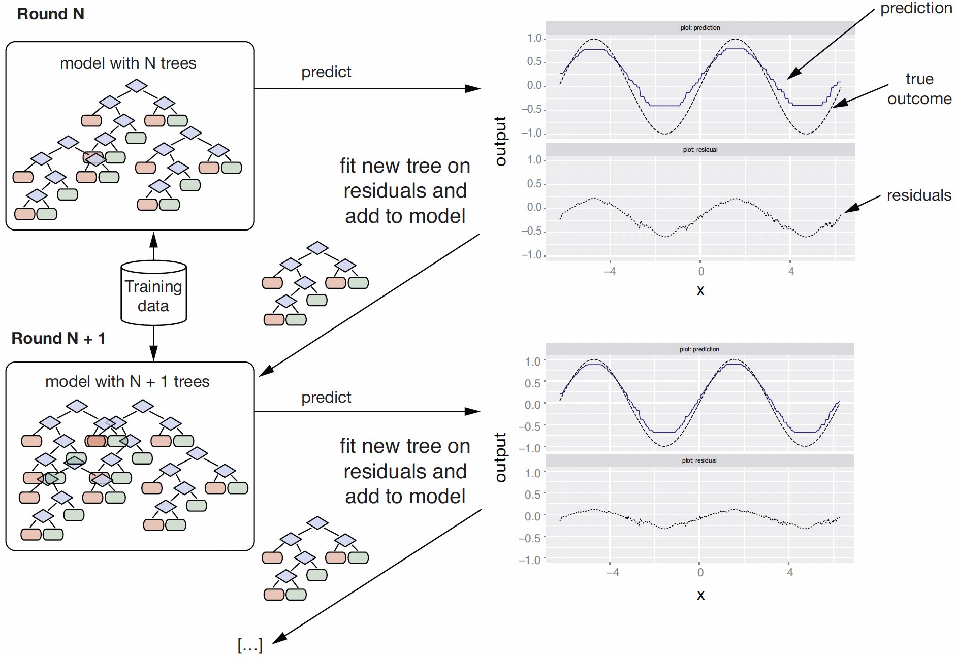
Building up a gradient-boosted tree model

Visual Example of Boosting in Action

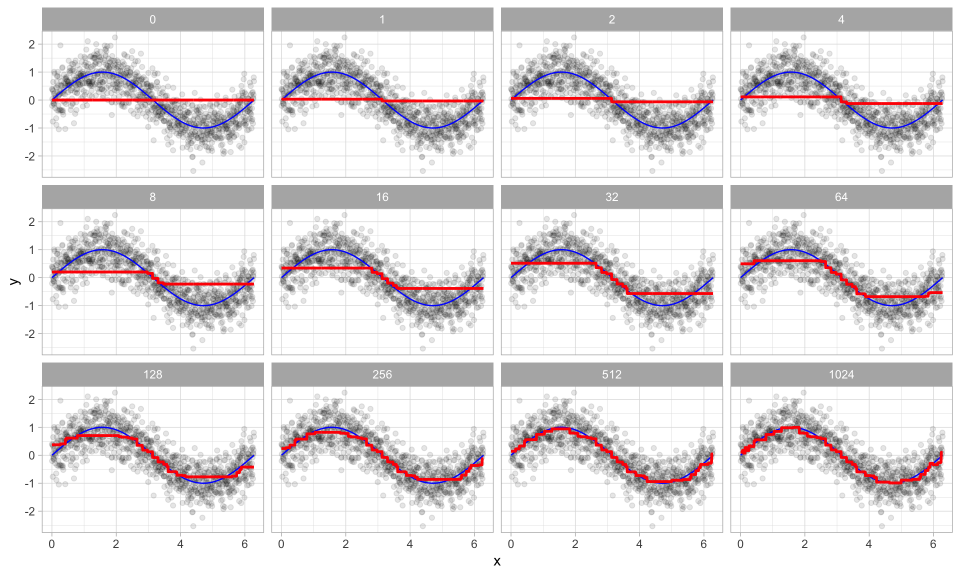
Boosted regression trees as 0-1024 successive trees are added.

What Is a “Gradient”?

Tip

• Think of the loss function as a hilly landscape.
• You are blindfolded at some starting point.
• The gradient tells you which direction is “uphill.”
• Gradient descent means: always take a step downhill.
• You keep going until you reach the valley floor (minimum loss).

• At each step, we calculate the gradient — the direction in which the loss increases most steeply — and move in the opposite direction.
• Adding each new tree moves the model one step downhill toward the minimum loss.

Gradient-Boosted Trees

Update the model parameters in the direction of the loss function (e.g., MSE, deviance)’s descending gradient

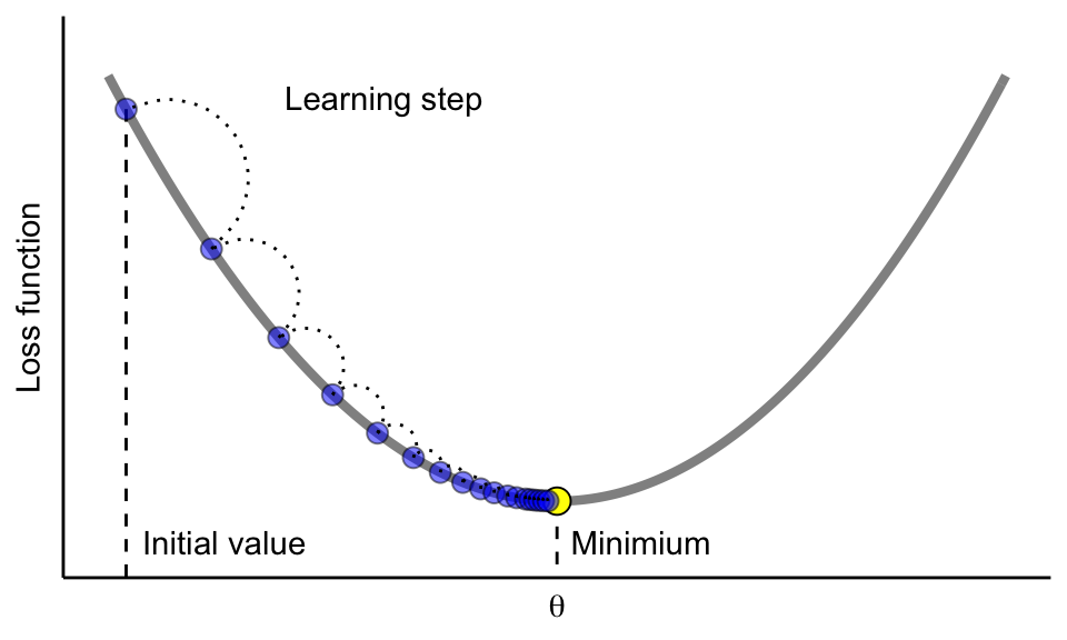
Tune the Learning Rate in Gradient Descent

We need to control how much we update by in each step - the learning rate

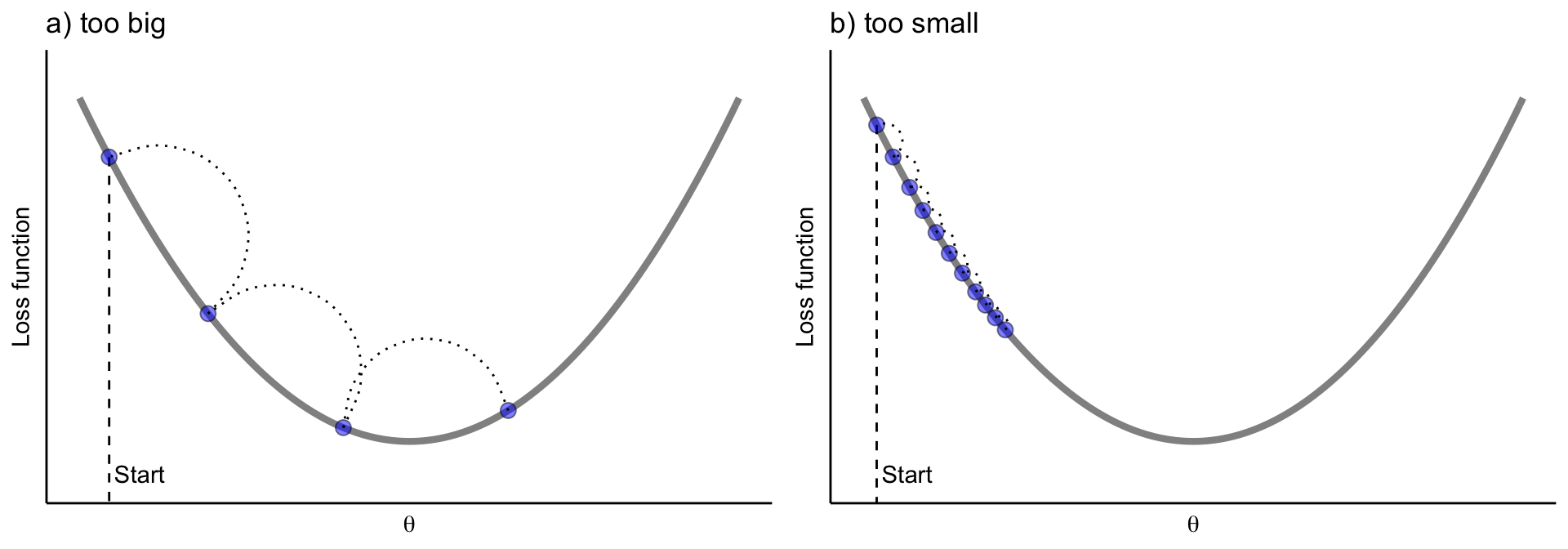
• Too large: overshoots the minimum — the model bounces back and forth and may never converge.
• Too small: takes tiny steps — eventually finds the minimum but requires far more trees and is slow.
• A good learning rate (eta) takes moderate, steady steps downhill to the minimum loss.

nrounds and eta Must Be Tuned Together

• A smaller eta (learning rate) means each tree contributes less, so you need more trees (nrounds) to reach good performance.
• A common strategy is to set eta small (e.g., 0.05–0.1) and then find the right nrounds via early stopping.

eXtreme Gradient Boosting with XGBoost

• XGBoost is one of the most popular open-source library for the gradient boosting algorithm.

Tuning hyperparameters with XGBoost

• number of trees (nrounds)
• learning rate (eta), i.e. how much we update in each step
• nrounds and eta really have to be tuned together
• complexity of the trees (max_depth, min_child_weight)
  • max_depth: the maximum depth a tree is allowed to grow. Larger values let the model capture more complex patterns, but can increase overfitting.
  • min_child_weight: the minimum total instance weight required in a child node for a split to be allowed. Larger values make the model more conservative by preventing splits that create very small or weakly supported nodes.
• XGBoost also provides more regularization (via gamma) and early stopping

Practical Tuning Guidance for XGBoost

Hyperparameter	Typical Starting Point	Effect of Increasing
nrounds	100–500 (with early stopping)	More trees; use early stopping to avoid overfitting
eta	0.05–0.1	Slower learning; needs more nrounds
max_depth	3–6	Deeper trees; captures more interactions but risks overfitting
min_child_weight	1–10	More conservative splits; reduces overfitting
gamma	0–1	Higher penalty for additional splits; simpler trees

A good default workflow: fix eta = 0.05, use early stopping to find the right nrounds, then tune max_depth and min_child_weight.

Random Forest vs. Gradient-Boosted Trees (1)

• Both are tree-based ensemble methods
  • They combine many trees to improve predictive performance over a single decision tree.
• Random forest builds trees independently
  • Each tree is grown separately using bootstrap samples and random subsets of predictors.
  • Because trees do not depend on each other, random forest can be trained in parallel.
• Gradient-boosted trees build trees sequentially
  • Each new tree is added to improve the errors made by the current ensemble.
  • Because each tree depends on the previous one, gradient boosting must be trained one step at a time.

Random Forest vs. Gradient-Boosted Trees (2)

• Random forest mainly reduces variance
  • Averaging many de-correlated trees helps make predictions more stable and less sensitive to overfitting.
• Gradient boosting mainly reduces bias
  • By repeatedly correcting errors, it can fit complex patterns more closely.
• Random forest is usually easier to tune
  • A few tuning choices such as mtry are often enough to get strong performance.
• Gradient-boosted trees usually require more careful tuning
  • We often need to tune nrounds, eta, tree depth, and other settings together.

Random Forest vs. Gradient-Boosted Trees — When to Use Which?

	Random Forest	Gradient-Boosted Trees (XGBoost)
How trees are built	Independently (parallel)	Sequentially (one at a time)
Main error reduced	Variance	Bias
Tuning effort	Low — mtry and ntree	Higher — eta, nrounds, max_depth, etc.
Risk of overfitting	Lower (averaging stabilizes)	Higher (can memorize with too many trees)
Typical performance	Strong, robust baseline	Often best-in-class on tabular data
Interpretability	Variable importance plots	Variable importance + partial dependence

Rule of thumb: Start with random forest for a quick, reliable baseline. Switch to XGBoost when you need to squeeze out maximum predictive accuracy and are willing to invest time in tuning.