Lecture 5

Tree-based Model I: Decision Trees

Byeong-Hak Choe

bchoe@geneseo.edu

SUNY Geneseo

March 23, 2026

Decision Trees

Decision Trees

• Decision trees partition training data into homogeneous nodes/subgroups with similar response values
  • Decision trees take any type of data, numerical or categorical.
• The subgroups are found recursively using binary partitions
  • i.e. asking a series of yes-no questions about the predictor variables
• We stop splitting the tree once a stopping criteria has been reached (e.g. maximum depth allowed)

Decision Tree Terminologies

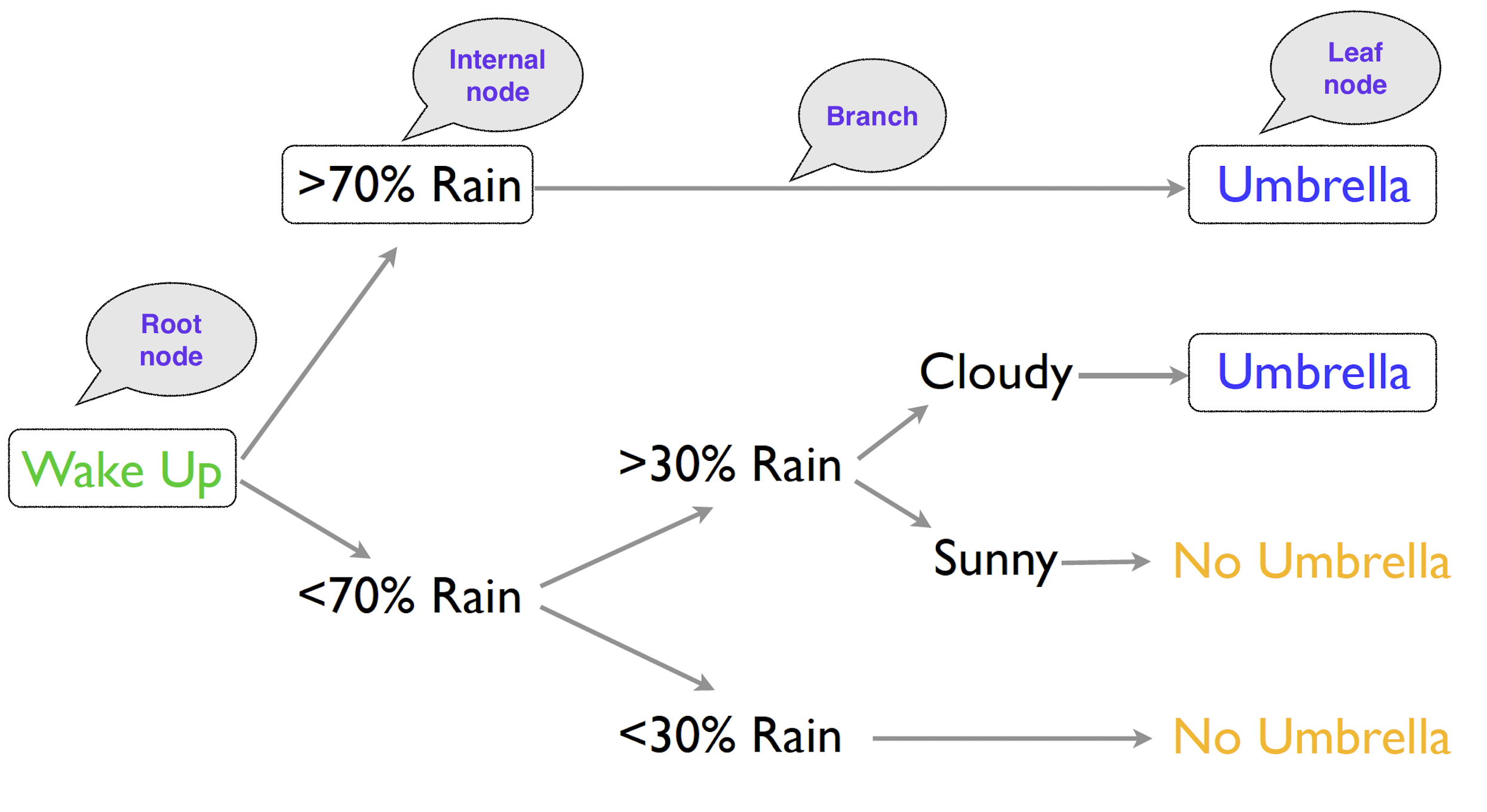
• Each decision is a node, and the final prediction is a leaf node.

Tree-logic

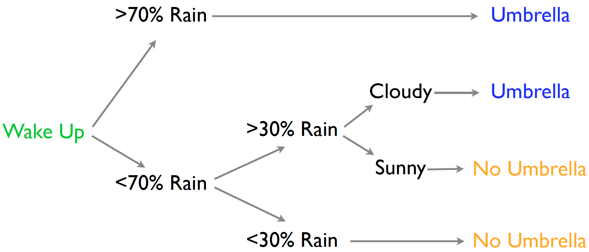
• Tree-logic uses a series of steps to come to a conclusion.
• The trick is to have mini-decisions combine for good choices.
• We make a prediction for an observation by following its path along the tree.

Classification and Regression Trees (CART)

• For each subgroup/node, predictions are made with:
  • Regression tree: the average of the outcome values in the node
  • Classification tree: the most popular class in the node
• Regression trees have a mean outcome at the leaves.
  • The expected amount of rain is 2.2 inches (so take an umbrella).
• Classification trees have class probabilities at the leaves.
  • Probability I’ll be in heavy rain is 0.9 (so take an umbrella).
• Decision trees make fewer assumptions about the relationship between x and y.
  • E.g., linear model assumes the linear relationship between x and y.
• Decision trees naturally express certain kinds of interactions among the predictor variables: those of the form: “IF x is true AND y is true, THEN….”

Regression Tree with NBC Shows

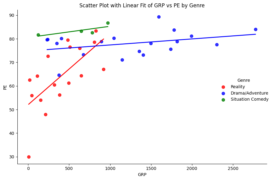
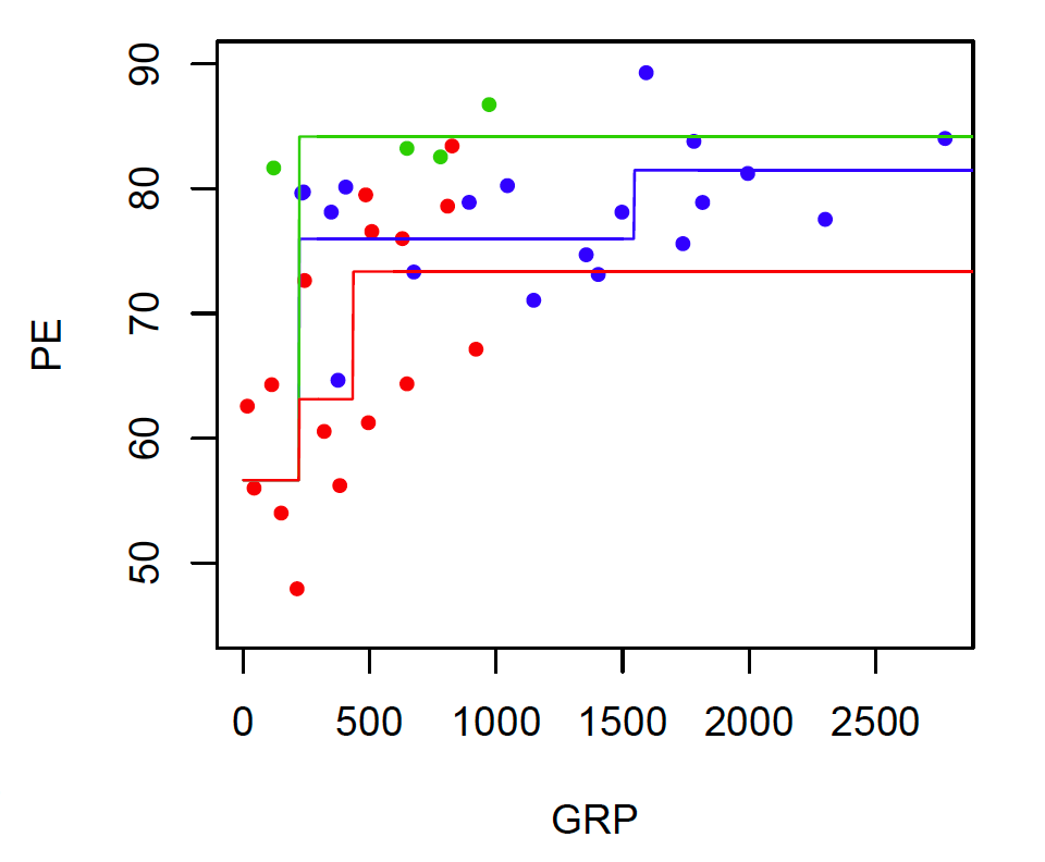
• Nonlinear: PE increases with GRP, but in jumps
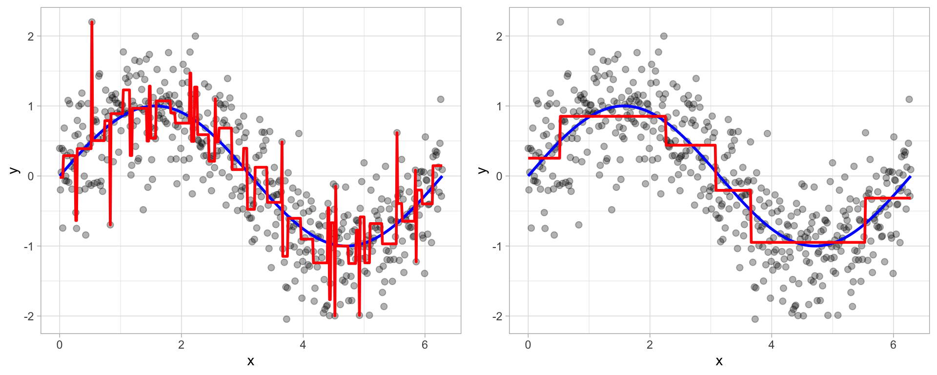
  • Trees automatically learn non-linear response functions and will discover interactions between predictors.
• This flexibility is helpful, but it also raises the risk of overfitting.

Fitting a Decision Tree

• We need a way to estimate the sequence of decisions:
  • which predictor to split on
  • where to split it
  • how many splits to keep
• CART grows the tree through a sequence of splits:
  1. Given any set (node) of data, you can find the optimal split (the error minimizing split) and divide into two child sets.
  2. We then look at each child set, and again find the optimal split to divide it into two homogeneous subsets.
  3. The children become parents, and we look again for the optimal split on their new children (the grandchildren!).
• You stop splitting and growing when the size of the leaf nodes hits some minimum threshold (e.g., say no less than 10 observations per leaf).

Fitting a Decision Tree: Recursive Splits

Each split/rule depends on the previous split/rule above it

Objective at each split: find the best predictor and cutoff to partition the data into two regions, \(R_1\) and \(R_2\), so that the predictions within each resulting node are as accurate as possible.

• For a regression tree, we choose the split that minimizes the sum of squared errors (SSE): \[ SSE = \sum_{i \in R_1} (y_i - c_1)^2 + \sum_{i \in R_2} (y_i - c_2)^2 \]

  • \(y_i\) is the actual response for observation \(i\)
  • \(c_1\) is the mean response among observations in region \(R_1\)
  • \(c_2\) is the mean response among observations in region \(R_2\)

Fitting a Decision Tree: Recursive Splits

Each split/rule depends on the previous split/rule above it

Objective at each split: find the best predictor and cutoff to partition the data into two regions, \(R_1\) and \(R_2\), so that the predictions within each resulting node are as accurate as possible.

• For a classification tree using the Gini index, we choose the split that minimizes the weighted impurity: \[ \frac{|R_1|}{|R_1| + |R_2|} \left( 1 - \sum_{k=1}^{K} p_{1k}^{2} \right) \;+\; \frac{|R_2|}{|R_1| + |R_2|} \left( 1 - \sum_{k=1}^{K} p_{2k}^{2} \right) \]
  • \(|R_i|\): the numbers of observations in regions \(R_i\) (\(i = 1, 2\))
  • \(p_{ik}\) is the proportion of observations in region \(R_i\) that belong to class \(k\)
  • \(K\) is the total number of classes

Fitting a Decision Tree: Recursive Splits

Each split/rule depends on previous split/rule above it

• Regression: each split is chosen to make the observations within each child node as similar as possible in their outcome values.

• Classfication: a good split makes each child node as pure as possible, meaning observations within each region mostly belong to one class.

• Splits yield locally optimal results, so we are NOT guaranteed to train a model that is globally optimal

• How do we control the complexity of the tree?

Tuning and Pruning Trees

Why complexity control matters

• A very small tree may underfit important structure in the data.
• A very large tree may fit noise rather than signal.
• Training error almost always improves as the tree grows.
• But prediction on new data may stop improving, or even worsen, when the tree becomes too complex.
• So the main question is not whether more splits improve in-sample fit. They usually do.
• The real question is whether additional splits improve out-of-sample prediction.

Important tuning choices for a single tree

• Maximum depth (maxdepth)
• Minimum number of observations required to split a node (minsplit)
• Minimum number of observations allowed in a terminal node (minbucket)
• Complexity parameter used for cost-complexity pruning (cp)

Bias-variance tradeoff in trees

• Too shallow: the tree may miss important nonlinearities and interactions.
• Too deep: the tree may react too strongly to random quirks in the training data.
• Simpler trees have more bias but less variance.
• More complex trees have less bias but more variance.
• Pruning is one way to move back toward a simpler tree after first allowing the tree to grow.

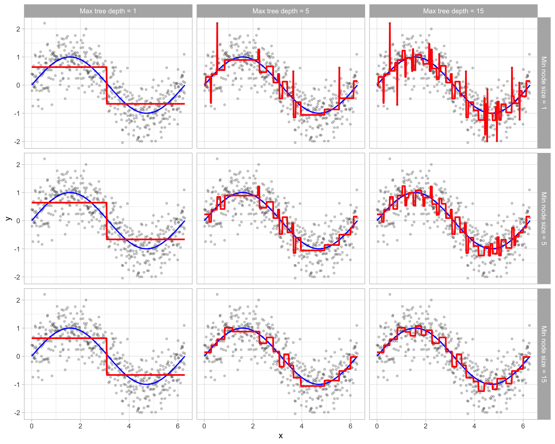
Tune the maximum tree depth or minimum node size

Prune the tree by tuning cost complexity

We can grow a very large complicated tree, and then prune back to an optimal subtree using a cost complexity parameter \(\alpha\) (like \(\lambda\) for regularization)

• \(\alpha\) penalizes objective as a function of the number of terminal nodes

• e.g., we want to minimize \(SSE + \alpha \cdot (\# \text{ of terminal nodes})\)

How to interpret the pruning penalty

• If \(\alpha = 0\), there is no direct penalty for complexity, so larger trees are favored.
• As \(\alpha\) increases, the model increasingly prefers smaller trees.
• Small values of \(\alpha\) allow more splits.
• Large values of \(\alpha\) remove more splits.
• In practice, we do not usually pick \(\alpha\) by pure intuition.
• Instead, we use cross-validation to estimate which pruning level generalizes best.

Pruning

• Trees are often grown large first, then cut back
• Pruning removes weak lower-level splits
• This produces a smaller subtree with better generalization
• Cross-validation is commonly used to choose the pruning level

Hyperparameter Tuning

• Hyperparameters are parameters set before training a model — unlike regular model parameters (e.g., coefficients), they are not learned from the data.

  • Examples include cp, minsplit, and minbucket in a decision tree.

• Hyperparameter tuning is the process of searching for the combination of hyperparameter values that produces the best model performance on unseen data.

• A model trained with poorly chosen hyperparameters tends to overfit (too complex) or underfit (too simple).

• Tuning finds the sweet spot that balances bias and variance.