Lecture 4

K-fold Cross-Validation; Bias-Variance Trade-off; Regularized Regression

Byeong-Hak Choe

bchoe@geneseo.edu

SUNY Geneseo

February 25, 2026

\(K\)-fold Cross-Validation

K-fold Cross-Validation

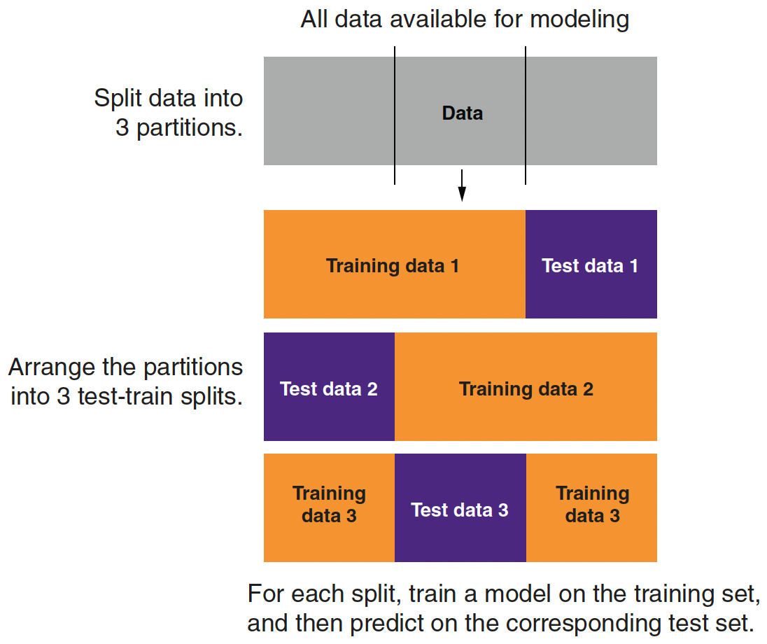
Partitioning Data for 3-fold Cross-Validation

• A single train–test split uses each subset only once—either for training or for evaluation.
• K‑fold cross-validation divides the training data into K equal parts (folds).
  • For each fold \(k=1, \dots, K\):
    • Step 1: Train the model on \(K‑1\) folds.
    • Step 2: Evaluate the model on the held‑out fold.
• The average error across folds provides a robust estimate of model performance.

Training, Validation, and Test Datasets

• Training Data:
  The portion of data used to fit the model.
  Within this set, k‑fold cross-validation is applied.

• Validation Data:
  Temporary splits within the training set during cross-validation, used to tune hyperparameters and assess performance.

• Test Data:
  A held-out dataset that is never used during model tuning.
  Provides an unbiased evaluation of the final model’s performance.

• Workflow:

  1. Split: Divide the dataset into training and test sets.
  2. Cross-Validate: Apply k‑fold CV on the training set for model tuning and selection.
  3. Evaluate: Use the test set for final performance assessment.

Bias-Variance Trade-off

Underfit vs. Optimal vs. Overfit

• Underfit: too simple, so it misses the main structure (systematic pattern) in the data.
  
• Optimal: complex enough to capture the overall trend, but not so flexible that it chases noise.
  
• Overfit: fits the training points extremely well, but the curve is too sensitive to small changes, so the shape is not stable and generalizes poorly.

Bias vs. Variance

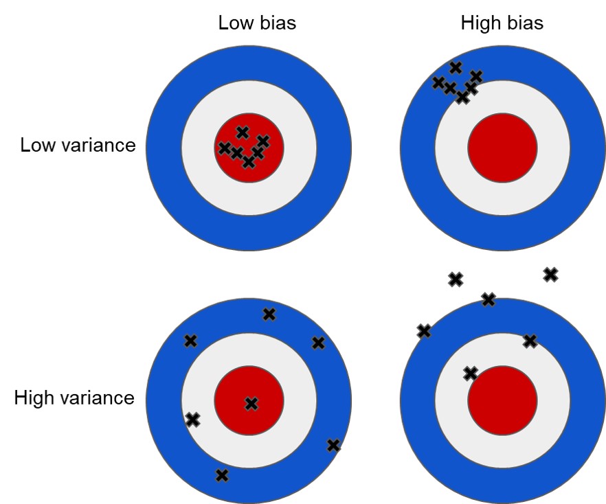
• Think of each black × as the model’s prediction from a different training sample.

• Low bias + low variance (top-left): accurate and stable → best generalization.
• High bias + low variance (top-right): stable but consistently wrong → underfitting.
• Low bias + high variance (bottom-left): right on average but noisy → overfitting risk.
• High bias + high variance (bottom-right): wrong and unstable → usually the worst case.

Why We Care

• Our real goal is good performance on new data, not perfect fit on the training data.
• When we make a model more flexible (more variables, higher-degree terms, complex interactions), two things move in opposite directions:
  • Bias tends to decrease (the model can match patterns better).
  • Variance tends to increase (the model becomes more sensitive to the particular training sample).

A Useful Decomposition (for Squared Error)

For a prediction \(\hat{y}\), the expected test MSE can be written as

\[ \text{(Error)}^{2} = \text{(Bias)}^{2} + \text{(Variance)} + \text{(Irreducible Noise)} \]

• Bias: how far the average prediction is from the truth (\(\widehat{y}\; - y\)).
• Variance: how much \(\widehat{y}\) would change if we collected a different training sample.
• Irreducible noise: randomness in \(y\) that no model can explain.

The Bias–Variance Trade-off Curve

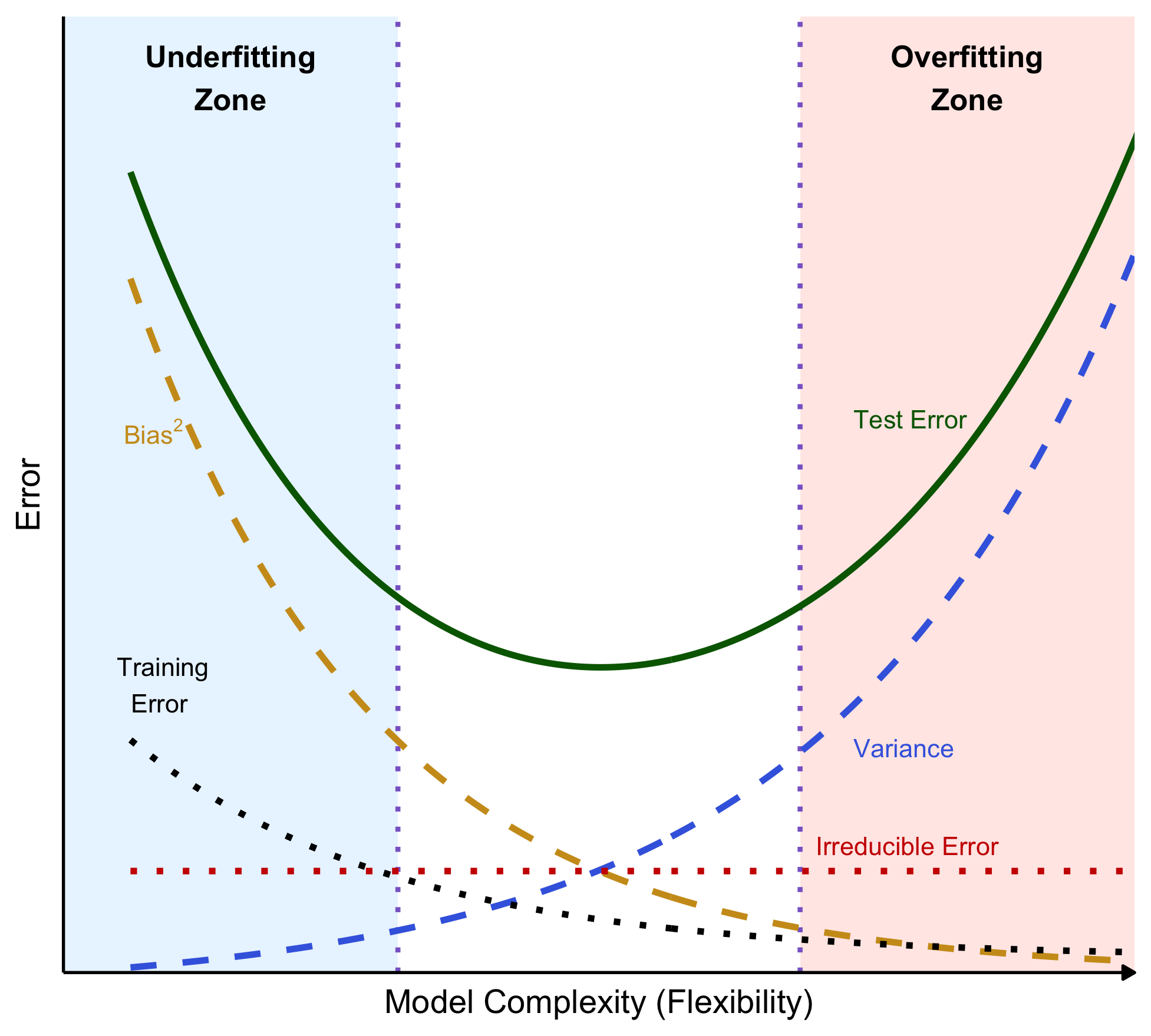
• Bias\(^2\): simple models cannot represent complex patterns → high systematic error
  • Adding flexibility lets the model capture real structure → lower bias
• Variance: flexible models adapt strongly to the specific training sample you happened to observe
  • if you re-sample the training data, the fitted model can change a lot

• The “best” complexity is near the bottom of the U (minimum test error).

Where Cross-Validation Fits

• We do not observe the “true” test error curve.
• K-fold cross-validation estimates out-of-sample error using only the training set.
• This lets us pick model settings that sit near the sweet spot in the bias-variance trade-off.

Where Cross-Validation Fits

• We do not observe the true Test MSE curve.
• K-fold cross-validation estimates out-of-sample performance using only the training data:
  \[ \text{CV Error} = \frac{1}{K}\sum_{k=1}^{K}\text{MSE}_k \]
• We repeat this for different model settings
• We then choose the settings with the lowest cross-validated error.
  • Increasing complexity usually reduces bias but increases variance.
  • Cross-validation helps us avoid both extremes by selecting a setting near the bias–variance sweet spot

Warning

• Cross-validation does not make the model “more accurate by itself.”
  • It is a selection procedure that helps us choose settings that are most likely to generalize well.

Regularization

Regularization

• Regularized regression can resolve the following problems:

  • Quasi-separation in logistic regression
  • Multicolinearity in linear regression
    • e.g., Variables \(\texttt{age}\) and \(\texttt{years_of_workforce}\) in linear regression of \(\texttt{income}\).
  • Overfitting (high variance)

• The above situations usually happen when the model is too complex (e.g., has large or many beta variables).

• We will discuss three regularized regression methods:

  • Lasso or LASSO (least absolute shrinkage and selection operator) (L1)
  • Ridge (L2)
  • Elastic net

What is Linear Regression Doing?

• Regular linear regression tries to find the beta parameters \(\beta_0, \beta_1, \beta_2, \,\cdots\, \beta_{p}\) such that \[ f(x_i) = b_0 + b_1 x_{1,i} + b_2 x_{2,i} + \,\cdots\, + b_p x_{p,i} \] is as close as possible to \(y_i\) for all the training data by minimizing the sum of the squared error (SSE) between \(y\) and \(f(x)\) with observations \(i = 1, \cdots, N\), where the SSE is \[ (y_1 - f(x_1))^2 + (y_2 - f(x_2))^2 + \,\cdots\, + (y_N - f(x_N))^2 \]

What is Lasso Regression Doing?

• Lasso regression tries to find the beta parameters \(\beta_0, \beta_1, \beta_2, \,\cdots\, \beta_{p}\) and \(\lambda\) such that \[ f(x_i) = b_0 + b_1 x_{1,i} + b_2 x_{2,i} + \,\cdots\, + b_p x_{p,i} \] is as close as possible to \(y_i\) for all the training data by minimizing the sum of the squared error (SSE) plus the sum of the absolute value of the beta parameters multiplied by the alpha parameter: \[ \begin{align} &(y_1 - f(x_1))^2 + (y_2 - f(x_2))^2 + \,\cdots\, + (y_N - f(x_N))^2 \\ &+ \lambda \times(| \beta_1 | + |\beta_2 | + \,\cdots\, + |\beta_{p}|) \end{align} \]
• When \(\lambda = 0\), this reduces to regular regression.

What is Lasso Regression Doing?

• When variables are nearly collinear, lasso regression tends to drive one or more of them to zero.

• In the regression of \(\text{income}\), lasso regression might give zero credit to one of the two variables, \(\texttt{age}\) and \(\texttt{years_of_workforce}\).

• For this reason, lasso regression is often used as a form of model/variable selection.

What is Ridge Regression Doing?

• Ridge regression tries to find the beta parameters \(\beta_0, \beta_1, \beta_2, \,\cdots\, \beta_{p}\) and \(\lambda\) such that \[ f(x_i) = b_0 + b_1 x_{1,i} + b_2 x_{2,i} + \,\cdots\, + b_p x_{p,i} \] is as close as possible to \(y_i\) for all the training data by minimizing the sum of the squared error (SSE) plus the sum of the squared beta parameters multiplied by the alpha parameter: \[ \begin{align} &(y_1 - f(x_1))^2 + (y_2 - f(x_2))^2 + \,\cdots\, + (y_N - f(x_N))^2 \\ &+ \lambda \times (\beta_1^2 + \beta_2^2 + \,\cdots\, + \beta_{p}^2) \end{align} \]
• When \(\lambda = 0\), this reduces to regular regression.

What is Ridge Regression Doing?

• When variables are nearly collinear, ridge regression tends to average the collinear variables together.
• You can think of this as “ridge regression shares the credit.”
  • Imagine that being one year older/one year longer in the workforce increases \(\texttt{income}\) in the training data.
  • In this situation, ridge regression might give a half credit to each variable of \(\texttt{age}\) and \(\texttt{years_of_workforce}\), which adds up to the appropriate effect.

What is Elastic Net Regression Doing?

• Elastic net regression tries to find the beta parameters \(\beta_0, \beta_1, \beta_2, \,\cdots\, \beta_{p}\), \(\alpha\), and \(\lambda\) such that \[ f(x_i) = b_0 + b_1 x_{1,i} + b_2 x_{2,i} + \,\cdots\, + b_p x_{p,i} \] is as close as possible to \(y_i\) for all the training data by minimizing the sum of the squared error (SSE) plus a linear combination of the ridge and the lasso penalties with the \(\alpha\) parameter: \[ \begin{align} &(y_1 - f(x_1))^2 + (y_2 - f(x_2))^2 + \,\cdots\, + (y_N - f(x_N))^2 \\ &+ \alpha \times \lambda \times(| \beta_1 | + |\beta_2 | + \,\cdots\, + |\beta_{p}|)\\ &+ (1-\alpha)\times \lambda \times(\beta_1^2 + \beta_2^2 + \,\cdots\, + \beta_{p}^2) \end{align} \] where \(0 \leq \alpha \leq 1\).

• When \(\alpha = 0\), this reduces to Lasso regression.

• When \(\alpha = 1\), this reduces to Ridge regression.

Choosing Between Lasso, Ridge, and Elastic Net

• In some situations, such as when you have a very large number of variables, many of which are correlated to each other, the lasso may be preferred.
• In other situations, like quasi-separability, the ridge solution may be preferred.
• When you are not sure which is the best approach, you can combine the two by using elastic net regression.
  • Different values of \(\alpha\) between 0 and 1 give different trade-offs between sharing the credit among correlated variables, and only keeping a subset of them.

How Expensive Is It To Make \(\beta\) Large?

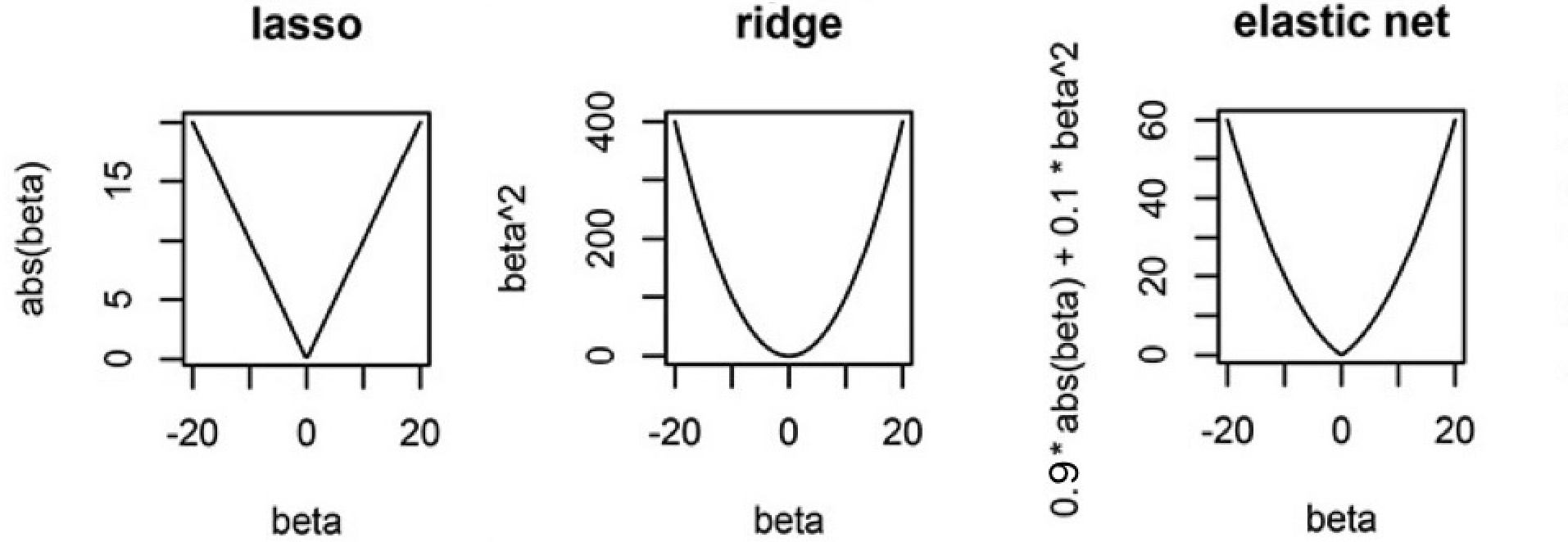
• Lasso (L1) Penalty (\(|\beta|\)):
  
  • Each unit increase in \(\beta\) adds a constant penalty, regardless of \(\beta\) ’s size.
  • Drives some coefficients exactly to zero, acting as a predictor selection mechanism.

• Ridge (L2) Penalty (\(\beta^2\)):
  
  • Gently penalizes small-to-moderate deviations from zero, but penalty increases quickly for large \(\beta\).
  • Shrinks coefficients but does not set them exactly to zero.

Intuition on Different Penalties

• The ellipses are contours of equal SSE (same fit quality).
• The shape is the constraint/penalty region.
  
• Lasso induces corner solutions!
• Lasso has corners, and corners create zeros.

Regularization Affects the Interpretation of Beta

• No Need to Omit a Reference Category:
  • In standard regression, one dummy is typically omitted to avoid perfect multicollinearity.
  • In regularized regression, the penalty term handles multicollinearity by shrinking all coefficients, so you can include all dummy variables.
  • Each coefficient then represents the deviation from a shared baseline (an implicit average effect).
• Interpretation:
  • With this approach, we interpret a dummy’s beta as how much that category’s association with the outcome, without worrying about the reference level (intercept).

Sparse Matrix

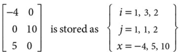
• R’s \(\texttt{glmnet}\) package uses a sparse matrix

• A sparse matrix is a matrix with many zero entries

• A sparse matrix is almost essential in big data analysis because of its lower storage costs and faster computation.

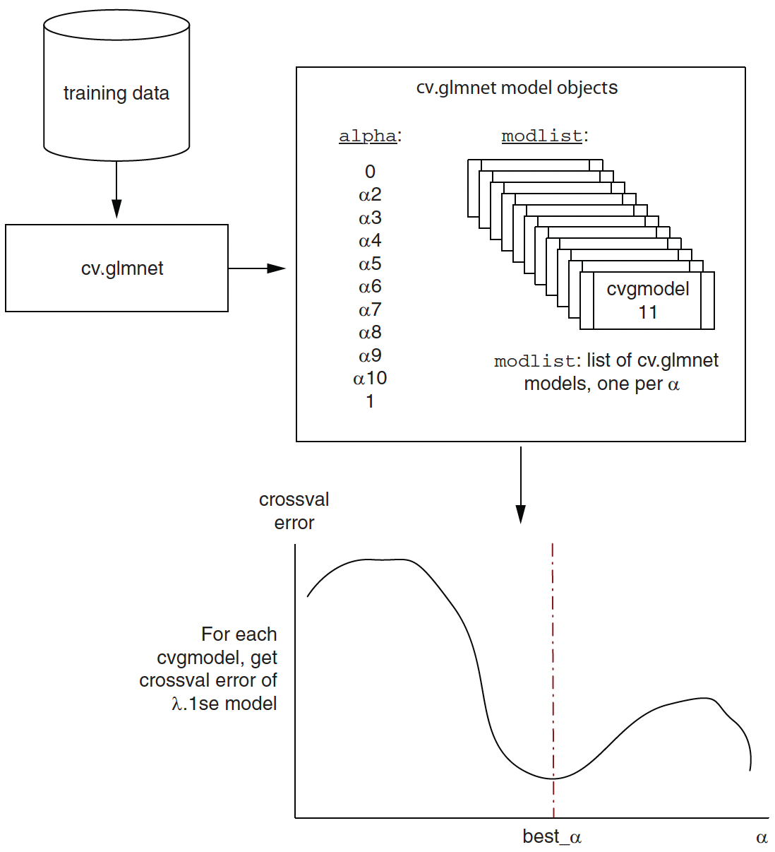
Lasso/Ridge Regression with Cross-Validation in R

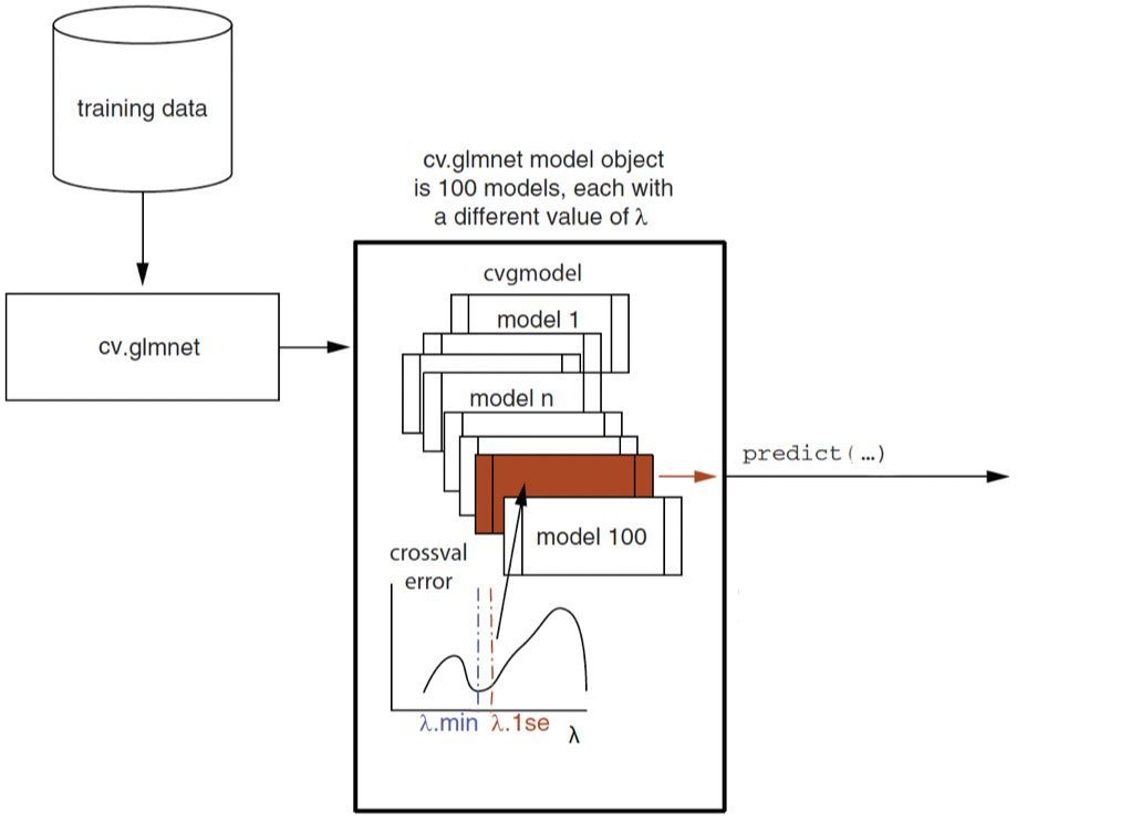
• \(\lambda_{min}\): the \(\lambda\) for the model with the minimum cross-validation (CV) error
• \(\lambda\texttt{.1se}\): corresponds to the model with cross-validation error, which is \(\textit{one standard error (se)}\) of CV error above the minimum CV error.

Elastic Net Regression with Cross-Validation in R

How Regularization Addresses the Bias-Variance Trade-off

• In regression, a common source of high variance is large and unstable coefficients (especially with many predictors or collinearity).
• Regularization adds a penalty for large coefficients.
  • This shrinks coefficients toward 0.
  • It usually increases bias a little but can reduce variance a lot.
• The result is often lower test error, even if training error gets slightly worse.

Practical rule of thumb about \(\lambda_{min}\) and \(\lambda\texttt{.1se}\)

• If you care most about predictive accuracy and don’t mind complexity: start with \(\lambda_{min}\).
• If you care about simplicity, interpretability, and stability: \(\lambda\texttt{.1se}\) is often the better default.

❌ Omitted Variable Bias

Omitted Variable Bias

• Omitted variable bias (OVB): bias in the model because of omitting an important regressor that is correlated with existing regressor(s).

• Let’s use an orange juice (OJ) example to demonstrate the OVB.

  • OJ price elasticity estimates vary with models, whether or not taking into account brand or ad_status

Variable	Description
sales	Quantity of OJ cartons sold
price	Price of OJ
brand	Brand of OJ
ad	Advertisement status

📏 Short- and Long- Regressions

• OVB is the difference in beta estimates between short- and long-form regressions.

• Short regression: The regression model with less regressors

\[ \begin{align} \log(\text{sales}_i) = \beta_0 + \beta_1\log(\text{price}_i) + \epsilon_i \end{align} \]

• Long regression: The regression model that adds additional regressor(s) to the short one.

\[ \begin{align} \log(\text{sales}_i) =& \beta_0 + \beta_{1}\log(\text{price}_i) \\ &+ \beta_{2}\text{minute.maid}_i + \beta_{3}\text{tropicana}_i + \epsilon_i \end{align} \]

• OVB for \(\beta_1\) is:

\[ \text{OVB} = \widehat{\beta_{1}^{short}} - \widehat{\beta_{1}^{long}} \]

OVB formula

• Consider the following short- and long- regressions:

  • Short: \(Y_i = \beta_0 + \beta_{1}^{short}X_1 + \epsilon_{short}\)
    
  • Long: \(Y_i = \beta_0 + \beta_{1}^{long}X_1 +\beta_{2}X_2 + \epsilon_{long}\)

• Error in short form can be represented as: \[ {\epsilon_{short}} = \beta_{2}X_2 + \epsilon_{long} \]

• If variable \(X_1\) is correlated with \(X_2\), the following assumptions are violated in the short regression model:

  • Errors are not correlated with regressors.
  • Errors have a mean value of 0.

❓🔍 How does an OVB happen in regression?

• In the first stage, consider the relationship between price and brand:

\[ \log(\text{price}) = \beta_0 + \beta_1\text{minute_maid} + \beta_2\text{tropicana} + \epsilon_{1st} \]

• Then, calculate the residual: \[ \widehat{\epsilon_{1st}} = \log(\text{price}) - \widehat{\log(\text{price})} \]

• The residual represents the log of OJ price after its correlation with brand has been removed!

• In the second stage, regress \(\log(\text{sales})\) on residual \(\widehat{\epsilon_{1st}}\):

\[ \log(\text{sales}) = \beta_0 + \beta_1\widehat{\epsilon_{1st}} + \epsilon_{2nd} \]

Regression Sensitivity Analysis

• Regression finds the coefficients on the part of each predictor that is independent from the other predictors.

• What can we do to deal with OVB problems?

  • Because we can never be sure whether a given set of controls is enough to eliminate OVB, it’s important to ask how sensitive regression results are to changes in the list of controls.