library(tidyverse)
library(scales)
library(broom)
library(stargazer)
library(glmnet)
library(janitor)
library(rpart)
library(rpart.plot)
library(ranger)
library(vip)
library(pdp)
library(DT)
library(rmarkdown)
library(hrbrthemes)
library(ggthemes)
library(xgboost)

theme_set(theme_ipsum())

scale_colour_discrete <- function(...) scale_color_colorblind(...)
scale_fill_discrete <- function(...) scale_fill_colorblind(...)Homework 4
Predicting Housing Price in California
Direction
- Please submit one Quarto Document of Homework 4 to Brightspace using the following file naming convention:
- Example:
danl-320-hw4-choe-byeonghak.qmd
- Example:
- Due: April 20, 2026, 11:59 P.M. (ET)
- Please send Byeong-Hak an email (
bchoe@geneseo.edu) if you have any questions.
Data
df <- read_csv('https://bcdanl.github.io/data/california_housing_cleaned.csv')- The housing data at census tract-level in California include:
- Latitude/longitude of tract centers
- Median home age
- Median income
- Average room/bedroom numbers
- Average occupancy
- Median home values
- The goal is to predict the log of median housing value for census tracts.
Question 1
- Divide the
dfDataFrame into training and test DataFrames.- Use
dtrainanddtestfor training and test DataFrames, respectively. - 70% of observations in the
dfare assigned todtrain; the rest is assigned todtest.
- Use
Show answer
set.seed(42120532)

df <- df |>
  mutate(rnd = runif(n()))

dtrain <- df |>
  filter(rnd >= .3)

dtest <- df |>
  filter(rnd < .3)

nrow(dtrain)
[1] 14366nrow(dtest)[1] 6274The training data contain 70% of the observations, and the test data contain the remaining 30%. I use set.seed() so that the random split is reproducible.
Question 2
- Consider the following model:
\[ \begin{align} \log(\text{medianHouseValue})_{i} = &\beta_0 + \beta_1 \text{housingMedianAge}_{i} + \beta_2 \text{medianIncome}_{i}\\ &+ \beta_3 \text{AveBedrms}_{i} + \beta_4 \text{AveRooms}_{i} + \beta_5 \text{AveOccupancy}_{i}\\ &+ \beta_{6}\text{longitude}_{i} + \beta_{7}\text{latitude}_{i} + \epsilon_{i} \end{align} \]
- Provide a rationale behind the model why it includes \(\text{longitude}\) and \(\text{latitude}\) as predictors for \(\log(\text{medianHouseValue})\).
Show answer
The model includes longitude and latitude because housing prices are strongly related to location. In California, census tracts near the coast, major cities, job centers, and high-amenity areas often have higher housing values than inland or less urban areas. Longitude and latitude provide a simple way to allow the model to account for broad spatial patterns in housing prices.
In other words, two census tracts with similar income, housing age, rooms, bedrooms, and occupancy may still have very different housing values because they are located in different parts of California. Including longitude and latitude helps reduce omitted-variable bias from location-related factors that are not directly measured in the dataset.
Question 3
- Fit the linear regression model in Question 2.
Show answer
lm_fit <- lm(
  log(medianHouseValue) ~ housingMedianAge + medianIncome +
    AveBedrms + AveRooms + AveOccupancy + longitude + latitude,
  data = dtrain
)

summary(lm_fit)
Call:
lm(formula = log(medianHouseValue) ~ housingMedianAge + medianIncome +
    AveBedrms + AveRooms + AveOccupancy + longitude + latitude,
    data = dtrain)

Residuals:
     Min       1Q   Median       3Q      Max
-2.58537 -0.21369 -0.00414  0.20567  1.98626

Coefficients:
                   Estimate Std. Error t value Pr(>|t|)
(Intercept)      -1.351e+01  3.862e-01 -34.988  < 2e-16 ***
housingMedianAge  2.104e-03  2.489e-04   8.454  < 2e-16 ***
medianIncome      1.881e-01  2.460e-03  76.465  < 2e-16 ***
AveBedrms         2.996e-01  1.781e-02  16.821  < 2e-16 ***
AveRooms         -3.932e-02  3.458e-03 -11.371  < 2e-16 ***
AveOccupancy     -1.378e-03  2.387e-04  -5.770 8.07e-09 ***
longitude        -2.935e-01  4.408e-03 -66.597  < 2e-16 ***
latitude         -2.918e-01  4.203e-03 -69.428  < 2e-16 ***
---
Signif. codes:  0 '***' 0.001 '**' 0.01 '*' 0.05 '.' 0.1 ' ' 1

Residual standard error: 0.3544 on 14358 degrees of freedom
Multiple R-squared:  0.6131,    Adjusted R-squared:  0.613
F-statistic: 3251 on 7 and 14358 DF, p-value: < 2.2e-16broom::tidy(lm_fit) |>
mutate(across(where(is.numeric), ~ round(.x, 4))) |>
paged_table()Question 4
- Interpret \(\hat{\beta_{2}}\), \(\hat{\beta_{4}}\), and \(\hat{\beta_{5}}\), obtained from the linear regression model in Question 3.
Show answer
lm_coef <- broom::tidy(lm_fit)

lm_coef |>
  filter(term %in% c("medianIncome", "AveRooms", "AveOccupancy")) |>
  mutate(
    percent_effect = 100 * (exp(estimate) - 1),
    across(where(is.numeric), ~ round(.x, 4))
  ) |>
  paged_table()
Because the dependent variable is \(\log(\text{medianHouseValue})\), the coefficients can be interpreted approximately as percentage changes in median housing value for a one-unit increase in the predictor, holding the other variables constant.
- \(\hat{\beta}_2\) on
medianIncome: A one-unit increase in median income is associated with an approximate 20.7% change in median housing value, holding other variables constant. SincemedianIncomeis measured in tens of thousands of dollars, this is a meaningful income-related price effect. - \(\hat{\beta}_4\) on
AveRooms: A one-unit increase in the average number of rooms per household is associated with an approximate -3.86% change in median housing value, holding other variables constant. - \(\hat{\beta}_5\) on
AveOccupancy: A one-unit increase in average occupancy is associated with an approximate -0.14% change in median housing value, holding other variables constant.
The exact percentage interpretation is \(100 \times [\exp(\hat\beta)-1]\) percent.
Questions 5-6
- Suppose the model allows for the relationship between the outcome and each of these predictors—\(\text{housingMedianAge}_{i}\), \(\text{medianIncome}_{i}\), \(\text{AveBedrms}_{i}\), \(\text{AveRooms}_{i}\), and \(\text{AveOccupancy}_{i}\)—to vary by location of Census tract.
\[ \begin{align} \log(\text{medianHouseValue})_{i} = &\beta_0 + \beta_1 \text{housingMedianAge}_{i} + \beta_2 \text{medianIncome}_{i}\\ &+ \beta_3 \text{AveBedrms}_{i} + \beta_4 \text{AveRooms}_{i} + \beta_5 \text{AveOccupancy}_{i}\\ &+ \beta_6 \text{longitude}_{i} + \beta_7 \text{latitude}_{i}\\ &+ (\beta_8 \text{housingMedianAge}_{i} + \beta_9 \text{medianIncome}_{i}\\ &\qquad+ \beta_{10} \text{AveBedrms}_{i} + \beta_{11} \text{AveRooms}_{i} + \beta_{12} \text{AveOccupancy}_{i} ) \times \text{longitude}_{i}\\ &+ (\beta_{13} \text{housingMedianAge}_{i} + \beta_{14} \text{medianIncome}_{i}\\ &\qquad+ \beta_{15} \text{AveBedrms}_{i} + \beta_{16} \text{AveRooms}_{i} + \beta_{17} \text{AveOccupancy}_{i} ) \times \text{latitude}_{i}\\ &+ (\beta_{18} \text{housingMedianAge}_{i} + \beta_{19} \text{medianIncome}_{i} \\ &\qquad+ \beta_{20} \text{AveBedrms}_{i} + \beta_{21} \text{AveRooms}_{i} + \beta_{22} \text{AveOccupancy}_{i} )\times \text{longitude}_{i} \times \text{latitude}_{i}\\ &+ \epsilon_{i} \end{align} \]
The following code creates the outcome vector and predictor matrices for the regularized regression models. I standardize the predictors so that the Lasso and Ridge penalties treat variables on comparable scales.
y_train <- log(dtrain$medianHouseValue)
y_test <- log(dtest$medianHouseValue)

x_train <- model.matrix(
  log(medianHouseValue) ~
    (housingMedianAge + medianIncome + AveBedrms + AveRooms + AveOccupancy) *
    longitude * latitude,
  data = dtrain
)[, -1]

x_test <- model.matrix(
  log(medianHouseValue) ~
    (housingMedianAge + medianIncome + AveBedrms + AveRooms + AveOccupancy) *
    longitude * latitude,
  data = dtest
)[, -1]
Question 5
Fit a Lasso linear regression model.
Show answer
set.seed(42120532)

lasso_fit <- cv.glmnet(
  x = x_train,
  y = y_train,
  alpha = 1,
  standardize = TRUE
)

plot(lasso_fit)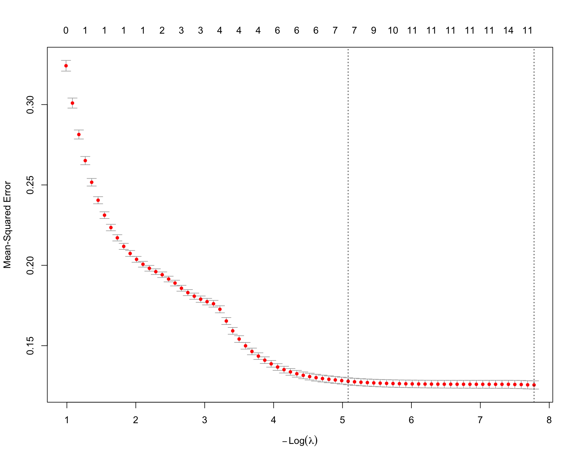
lasso_fit$lambda.min[1] 0.0004182971lasso_fit$lambda.1se[1] 0.006211579lasso_coefs <- coef(lasso_fit, s = "lambda.min")
lasso_coef_df <- tibble(
term = rownames(lasso_coefs),
estimate = as.numeric(lasso_coefs)
) |>
filter(estimate != 0,
!str_detect(term, "Intercept"))
lasso_coef_df |>
mutate(estimate = round(estimate, 4)) |>
arrange(-estimate) |>
paged_table()lasso_coef_df |>
mutate(estimate = round(estimate, 4)) |>
arrange(estimate) |>
paged_table()The Lasso model uses an \(L_1\) penalty, so some coefficients are shrunk exactly to zero. This is useful here because the interaction model contains many terms, and Lasso can select a smaller set of useful predictors.
Question 6
Fit a Ridge linear regression model.
Show answer
set.seed(42120532)

ridge_fit <- cv.glmnet(
  x = x_train,
  y = y_train,
  alpha = 0,
  standardize = TRUE
)

plot(ridge_fit)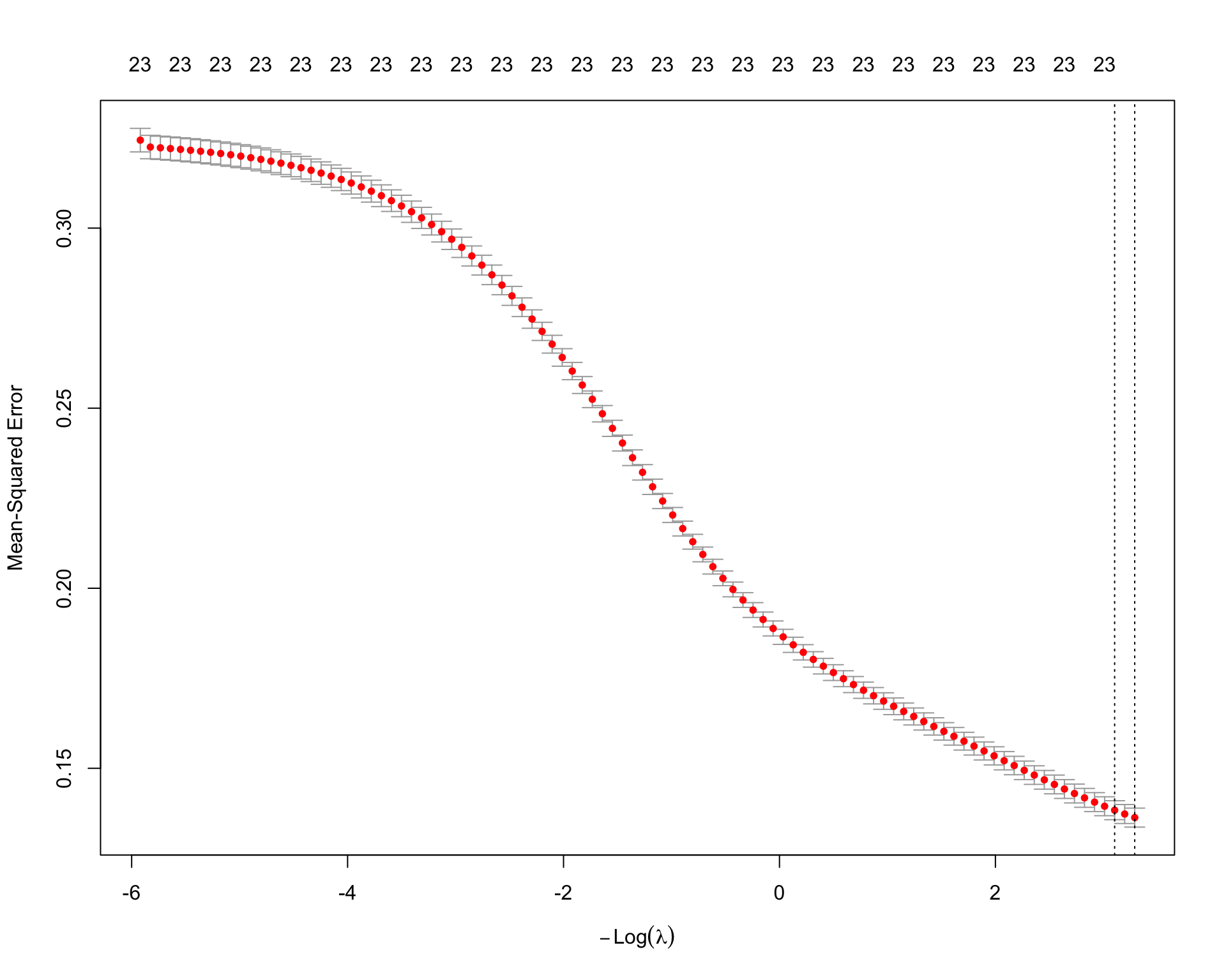
ridge_fit$lambda.min[1] 0.03723744ridge_fit$lambda.1se[1] 0.04485262ridge_coefs <- coef(ridge_fit, s = "lambda.min")
ridge_coef_df <- tibble(
term = rownames(ridge_coefs),
estimate = as.numeric(ridge_coefs)
) |>
filter(!str_detect(term, "Intercept"))
ridge_coef_df |>
mutate(estimate = round(estimate, 4)) |>
arrange(-estimate) |>
paged_table()ridge_coef_df |>
mutate(estimate = round(estimate, 4)) |>
arrange(estimate) |>
paged_table()The Ridge model uses an \(L_2\) penalty. Unlike Lasso, Ridge usually does not set coefficients exactly equal to zero. Instead, it shrinks all coefficients toward zero. This can improve prediction when many predictors and interaction terms are correlated.
Questions 7-10
Consider the tree-based model described below:
\[ \begin{align} \log(\text{medianHouseValue})_{i} = f(&\text{housingMedianAge}_{i}, \text{medianIncome}_{i},\\ &\text{AveBedrms}_{i}, \text{AveRooms}_{i}, \text{AveOccupancy}_{i},\\ &\text{latitude}_{i}, \text{longitude}_{i}) \end{align} \]
For tree-based models, I do not manually include interaction terms because trees can capture nonlinearities and interactions through recursive splitting.
tree_formula <- log(medianHouseValue) ~ housingMedianAge + medianIncome +
  AveBedrms + AveRooms + AveOccupancy + latitude + longitude
Question 7
Fit a regression tree model.
Show answer
set.seed(42120532)

tree_fit <- rpart(
  formula = tree_formula,
  data = dtrain,
  method = "anova",
  control = rpart.control(cp = 0, xval = 10, minsplit = 500)
)

tree_fit
n= 14366
node), split, n, deviance, yval
* denotes terminal node
1) root 14366 4660.419000 12.08645
2) medianIncome< 3.65675 7667 1989.847000 11.79333
4) medianIncome< 2.4184 3075 775.950600 11.56558
8) AveRooms>=3.906236 2088 408.183700 11.42515
16) latitude>=34.445 1349 232.700900 11.31813
32) longitude>=-119.905 373 31.751650 11.04943 *
33) longitude< -119.905 976 163.726600 11.42082
66) latitude>=39.355 236 17.827210 11.20071 *
67) latitude< 39.355 740 130.819600 11.49101
134) longitude>=-121.695 473 69.516660 11.38292 *
135) longitude< -121.695 267 45.986270 11.68250 *
17) latitude< 34.445 739 131.825500 11.62052
34) longitude>=-117.355 348 54.115870 11.43897 *
35) longitude< -117.355 391 56.031500 11.78210 *
9) AveRooms< 3.906236 987 239.489600 11.86265
18) AveRooms>=3.290162 577 112.741500 11.74517
36) medianIncome< 1.829 234 44.714740 11.58079 *
37) medianIncome>=1.829 343 57.390170 11.85732 *
19) AveRooms< 3.290162 410 107.579400 12.02797 *
5) medianIncome>=2.4184 4592 947.581100 11.94584
10) AveOccupancy>=2.294861 3578 590.727100 11.85160
20) AveRooms>=4.72801 2183 361.389400 11.73954
40) latitude>=34.47 1396 224.161600 11.64660
80) longitude>=-120.095 356 27.677380 11.36138 *
81) longitude< -120.095 1040 157.609500 11.74424
162) latitude>=38.465 431 41.241040 11.56033 *
163) latitude< 38.465 609 91.475700 11.87439
326) longitude>=-121.375 297 31.106140 11.69850 *
327) longitude< -121.375 312 42.435640 12.04182 *
41) latitude< 34.47 787 103.783800 11.90439
82) longitude>=-117.765 424 38.118600 11.71553 *
83) longitude< -117.765 363 32.877240 12.12498 *
21) AveRooms< 4.72801 1395 159.024300 12.02696
42) AveOccupancy>=3.255958 630 48.280980 11.92965
84) AveBedrms< 1.015509 255 21.867330 11.86604 *
85) AveBedrms>=1.015509 375 24.680590 11.97290 *
43) AveOccupancy< 3.255958 765 99.863530 12.10710
86) medianIncome< 3.09895 464 67.356880 12.03789 *
87) medianIncome>=3.09895 301 26.856500 12.21381 *
11) AveOccupancy< 2.294861 1014 212.936700 12.27839
22) latitude>=37.905 167 18.712250 11.92323 *
23) latitude< 37.905 847 169.005100 12.34842
46) housingMedianAge< 21.5 236 44.968910 12.09087 *
47) housingMedianAge>=21.5 611 102.335200 12.44790
94) AveOccupancy>=2.042897 291 47.897320 12.32546 *
95) AveOccupancy< 2.042897 320 46.108400 12.55924 *
3) medianIncome>=3.65675 6699 1257.886000 12.42193
6) medianIncome< 5.7093 4789 743.776700 12.28167
12) AveOccupancy>=2.684096 2863 320.258200 12.15977
24) medianIncome< 4.54095 1516 167.695200 12.05407
48) housingMedianAge< 41.5 1349 135.535600 12.02490
96) latitude>=34.475 546 75.450900 11.94729
192) longitude>=-121.685 313 37.867350 11.80078 *
193) longitude< -121.685 233 21.840550 12.14410 *
97) latitude< 34.475 803 54.559710 12.07767
194) longitude>=-117.795 289 20.755880 11.91718 *
195) longitude< -117.795 514 22.174250 12.16791
390) AveOccupancy>=3.251254 246 8.207118 12.07371 *
391) AveOccupancy< 3.251254 268 9.780243 12.25438 *
49) housingMedianAge>=41.5 167 21.737890 12.28972 *
25) medianIncome>=4.54095 1347 116.563600 12.27873
50) housingMedianAge< 18.5 462 40.688760 12.17451 *
51) housingMedianAge>=18.5 885 68.236390 12.33314
102) AveOccupancy>=2.974856 518 34.209510 12.27787
204) medianIncome< 5.1951 321 21.957820 12.22987 *
205) medianIncome>=5.1951 197 10.306530 12.35610 *
103) AveOccupancy< 2.974856 367 30.211750 12.41114 *
13) AveOccupancy< 2.684096 1926 317.729100 12.46288
26) latitude>=37.935 282 31.085760 12.12320 *
27) latitude< 37.935 1644 248.524200 12.52115
54) housingMedianAge< 19.5 431 61.891610 12.29196 *
55) housingMedianAge>=19.5 1213 155.949000 12.60259
110) AveOccupancy>=2.207103 846 95.234920 12.50752
220) medianIncome< 4.61895 494 59.078440 12.42365 *
221) medianIncome>=4.61895 352 27.805470 12.62522 *
111) AveOccupancy< 2.207103 367 35.443100 12.82173 *
7) medianIncome>=5.7093 1910 183.702900 12.77359
14) medianIncome< 7.60715 1304 110.215100 12.66807
28) AveOccupancy>=2.655956 873 61.672220 12.58860
56) medianIncome< 6.51565 527 34.401160 12.51564
112) housingMedianAge< 25.5 348 18.779550 12.45863 *
113) housingMedianAge>=25.5 179 12.291150 12.62649 *
57) medianIncome>=6.51565 346 20.193290 12.69973 *
29) AveOccupancy< 2.655956 431 31.862200 12.82904 *
15) medianIncome>=7.60715 606 27.726530 13.00065
30) housingMedianAge< 18.5 181 9.822655 12.89256 *
31) housingMedianAge>=18.5 425 14.888910 13.04668 *printcp(tree_fit)
Regression tree:
rpart(formula = tree_formula, data = dtrain, method = "anova",
    control = rpart.control(cp = 0, xval = 10, minsplit = 500))

Variables actually used in tree construction:
[1] AveBedrms        AveOccupancy     AveRooms         housingMedianAge
[5] latitude         longitude        medianIncome

Root node error: 4660.4/14366 = 0.32441

n= 14366

           CP nsplit rel error  xerror      xstd
1  0.30312421      0   1.00000 1.00010 0.0104105
2  0.07089626      1   0.69688 0.70200 0.0080118
3  0.05714406      2   0.62598 0.62879 0.0077844
4  0.03088077      3   0.56884 0.57691 0.0074129
5  0.02752483      4   0.53795 0.55629 0.0073371
6  0.02269955      5   0.51043 0.52418 0.0071493
7  0.01508736      6   0.48773 0.50585 0.0070944
8  0.00981913      7   0.47264 0.49650 0.0070257
9  0.00936770      8   0.46282 0.46735 0.0069895
10 0.00817934      9   0.45346 0.45467 0.0068650
11 0.00798697     10   0.44528 0.44322 0.0067568
12 0.00775882     11   0.43729 0.44005 0.0067121
13 0.00772450     13   0.42177 0.44005 0.0067121
14 0.00703542     14   0.41405 0.43432 0.0066561
15 0.00658388     15   0.40701 0.42923 0.0066215
16 0.00542246     16   0.40043 0.42155 0.0065850
17 0.00541140     17   0.39501 0.41540 0.0065250
18 0.00534132     18   0.38959 0.41520 0.0065356
19 0.00465644     19   0.38425 0.41164 0.0065162
20 0.00465153     20   0.37960 0.40537 0.0064377
21 0.00411309     21   0.37495 0.40368 0.0064614
22 0.00384814     22   0.37083 0.39952 0.0064663
23 0.00357923     23   0.36698 0.39744 0.0064626
24 0.00326113     24   0.36340 0.39073 0.0064159
25 0.00233451     26   0.35688 0.38260 0.0063855
26 0.00232379     27   0.35455 0.37521 0.0063678
27 0.00228233     31   0.34525 0.37522 0.0063663
28 0.00179190     32   0.34297 0.37431 0.0063582
29 0.00178727     33   0.34118 0.37326 0.0063485
30 0.00163901     34   0.33939 0.37083 0.0063437
31 0.00151870     35   0.33775 0.36879 0.0063428
32 0.00121237     36   0.33623 0.36595 0.0063348
33 0.00089839     37   0.33502 0.36365 0.0063188
34 0.00081862     38   0.33412 0.36238 0.0063013
35 0.00071462     39   0.33330 0.36183 0.0063026
36 0.00064693     40   0.33259 0.36162 0.0063030
37 0.00041738     41   0.33194 0.36158 0.0063101
38 0.00037187     42   0.33153 0.36166 0.0063115
39 0.00000000 43 0.33115 0.36161 0.0063103plotcp(tree_fit)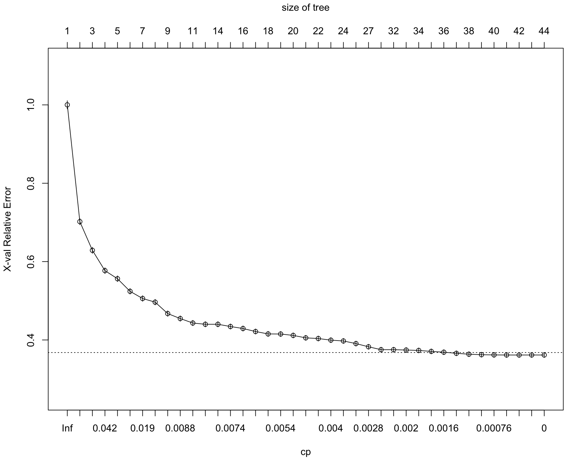
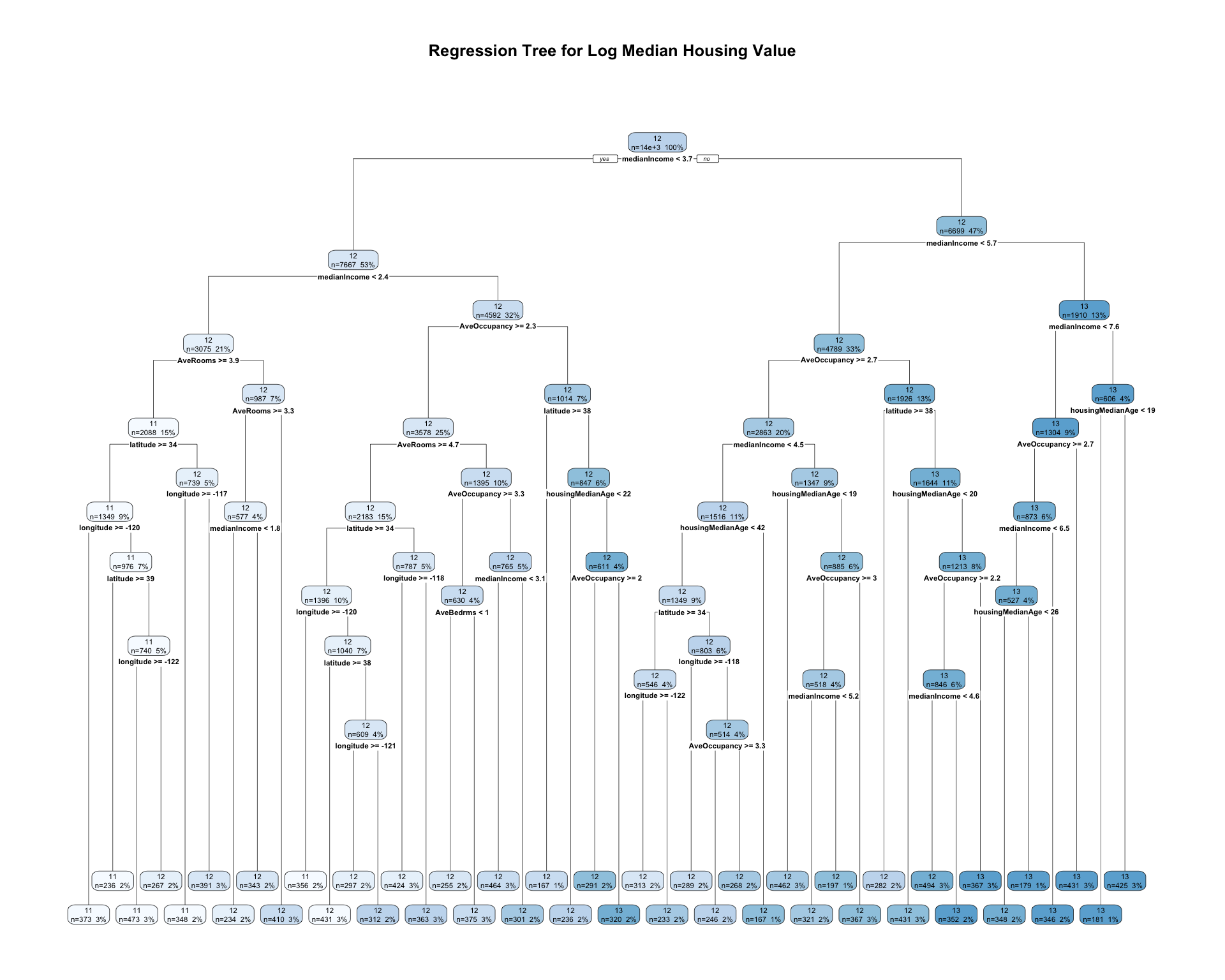
rpart.plot(
  tree_fit,
  type = 2,
  extra = 101,
  fallen.leaves = TRUE,
  main = "Regression Tree for Log Median Housing Value"
)
Prunning
cp_table <- tree_fit$cptable |>
  as_tibble()

min_row <- cp_table |>
  filter(xerror == min(xerror)) |>
  slice(1)

threshold <- min_row$xerror + min_row$xstd

best_cp_1se <- cp_table |>
  filter(xerror <= threshold) |>
  slice(1) |>
  pull(CP)

tree_pruned <- prune(tree_fit, cp = best_cp_1se)

tree_pruned
n= 14366
node), split, n, deviance, yval
* denotes terminal node
1) root 14366 4660.41900 12.08645
2) medianIncome< 3.65675 7667 1989.84700 11.79333
4) medianIncome< 2.4184 3075 775.95060 11.56558
8) AveRooms>=3.906236 2088 408.18370 11.42515
16) latitude>=34.445 1349 232.70090 11.31813
32) longitude>=-119.905 373 31.75165 11.04943 *
33) longitude< -119.905 976 163.72660 11.42082
66) latitude>=39.355 236 17.82721 11.20071 *
67) latitude< 39.355 740 130.81960 11.49101
134) longitude>=-121.695 473 69.51666 11.38292 *
135) longitude< -121.695 267 45.98627 11.68250 *
17) latitude< 34.445 739 131.82550 11.62052
34) longitude>=-117.355 348 54.11587 11.43897 *
35) longitude< -117.355 391 56.03150 11.78210 *
9) AveRooms< 3.906236 987 239.48960 11.86265
18) AveRooms>=3.290162 577 112.74150 11.74517
36) medianIncome< 1.829 234 44.71474 11.58079 *
37) medianIncome>=1.829 343 57.39017 11.85732 *
19) AveRooms< 3.290162 410 107.57940 12.02797 *
5) medianIncome>=2.4184 4592 947.58110 11.94584
10) AveOccupancy>=2.294861 3578 590.72710 11.85160
20) AveRooms>=4.72801 2183 361.38940 11.73954
40) latitude>=34.47 1396 224.16160 11.64660
80) longitude>=-120.095 356 27.67738 11.36138 *
81) longitude< -120.095 1040 157.60950 11.74424
162) latitude>=38.465 431 41.24104 11.56033 *
163) latitude< 38.465 609 91.47570 11.87439
326) longitude>=-121.375 297 31.10614 11.69850 *
327) longitude< -121.375 312 42.43564 12.04182 *
41) latitude< 34.47 787 103.78380 11.90439
82) longitude>=-117.765 424 38.11860 11.71553 *
83) longitude< -117.765 363 32.87724 12.12498 *
21) AveRooms< 4.72801 1395 159.02430 12.02696
42) AveOccupancy>=3.255958 630 48.28098 11.92965 *
43) AveOccupancy< 3.255958 765 99.86353 12.10710 *
11) AveOccupancy< 2.294861 1014 212.93670 12.27839
22) latitude>=37.905 167 18.71225 11.92323 *
23) latitude< 37.905 847 169.00510 12.34842
46) housingMedianAge< 21.5 236 44.96891 12.09087 *
47) housingMedianAge>=21.5 611 102.33520 12.44790
94) AveOccupancy>=2.042897 291 47.89732 12.32546 *
95) AveOccupancy< 2.042897 320 46.10840 12.55924 *
3) medianIncome>=3.65675 6699 1257.88600 12.42193
6) medianIncome< 5.7093 4789 743.77670 12.28167
12) AveOccupancy>=2.684096 2863 320.25820 12.15977
24) medianIncome< 4.54095 1516 167.69520 12.05407
48) housingMedianAge< 41.5 1349 135.53560 12.02490
96) latitude>=34.475 546 75.45090 11.94729
192) longitude>=-121.685 313 37.86735 11.80078 *
193) longitude< -121.685 233 21.84055 12.14410 *
97) latitude< 34.475 803 54.55971 12.07767
194) longitude>=-117.795 289 20.75588 11.91718 *
195) longitude< -117.795 514 22.17425 12.16791 *
49) housingMedianAge>=41.5 167 21.73789 12.28972 *
25) medianIncome>=4.54095 1347 116.56360 12.27873
50) housingMedianAge< 18.5 462 40.68876 12.17451 *
51) housingMedianAge>=18.5 885 68.23639 12.33314 *
13) AveOccupancy< 2.684096 1926 317.72910 12.46288
26) latitude>=37.935 282 31.08576 12.12320 *
27) latitude< 37.935 1644 248.52420 12.52115
54) housingMedianAge< 19.5 431 61.89161 12.29196 *
55) housingMedianAge>=19.5 1213 155.94900 12.60259
110) AveOccupancy>=2.207103 846 95.23492 12.50752
220) medianIncome< 4.61895 494 59.07844 12.42365 *
221) medianIncome>=4.61895 352 27.80547 12.62522 *
111) AveOccupancy< 2.207103 367 35.44310 12.82173 *
7) medianIncome>=5.7093 1910 183.70290 12.77359
14) medianIncome< 7.60715 1304 110.21510 12.66807
28) AveOccupancy>=2.655956 873 61.67222 12.58860
56) medianIncome< 6.51565 527 34.40116 12.51564 *
57) medianIncome>=6.51565 346 20.19329 12.69973 *
29) AveOccupancy< 2.655956 431 31.86220 12.82904 *
15) medianIncome>=7.60715 606 27.72653 13.00065 *rpart.plot(
tree_pruned,
type = 2,
extra = 101,
fallen.leaves = TRUE,
main = "Pruned Regression Tree for Log Median Housing Value"
)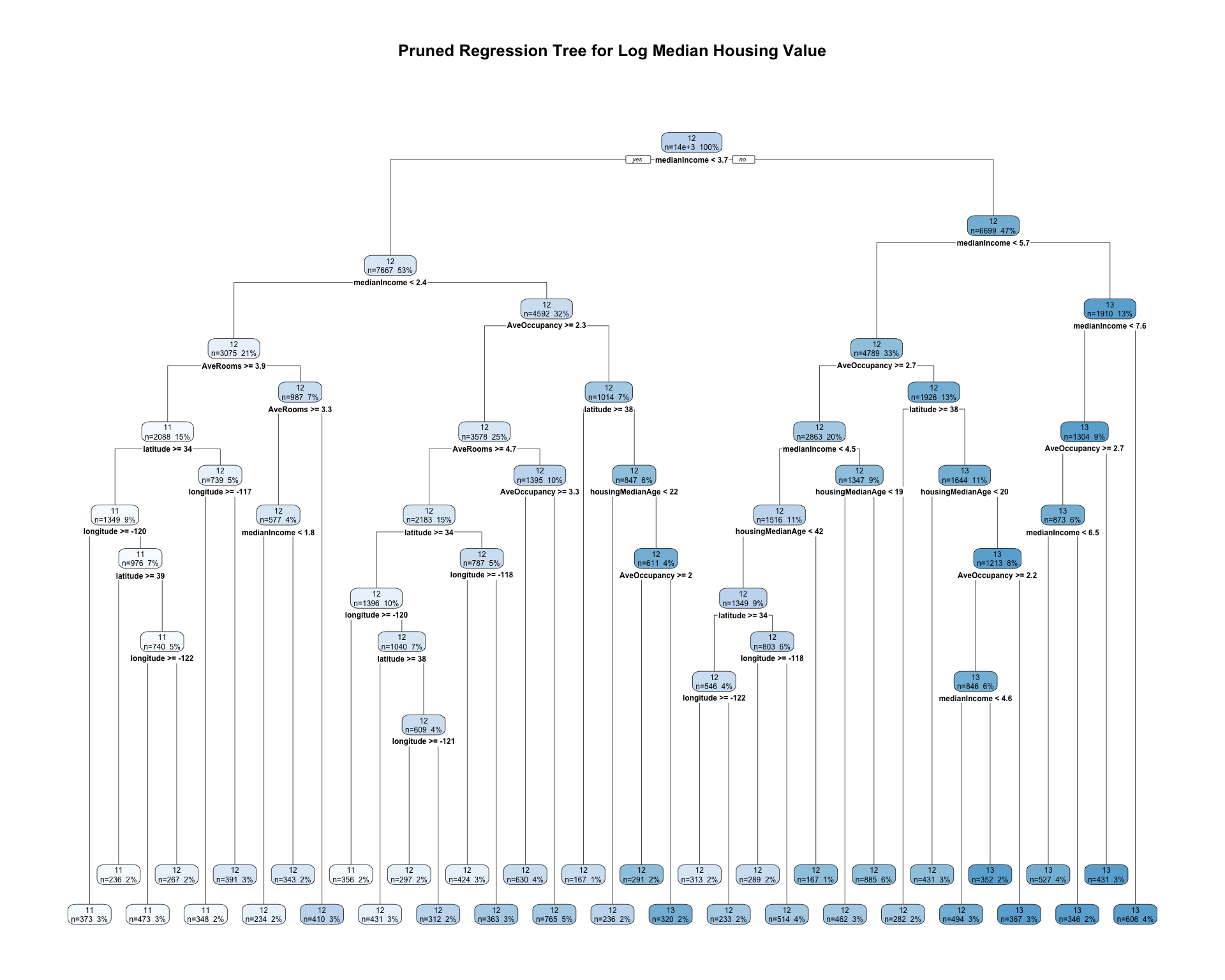
The initial regression tree is grown relatively flexibly by using a very small complexity parameter. This allows the tree to search for many possible splits in the training data. However, a large tree may overfit the training sample.
To reduce overfitting, I use the cost-complexity pruning table from rpart. The pruning parameter is selected based on the cross-validated error, xerror. The pruned tree keeps only the splits that improve predictive performance enough to justify the added complexity.
The pruned regression tree divides census tracts into groups using predictor values such as median income, housing characteristics, and location. Each terminal node predicts the average log median housing value for observations in that node. Compared with the full tree, the pruned tree is simpler and easier to interpret while still capturing important nonlinear patterns in the data.
Question 8
Fit a random forest model with num.trees = 500.
Show answer
set.seed(42120532)

rf_fit <- ranger(
  formula = tree_formula,
  data = dtrain,
  num.trees = 500,
  importance = "permutation"
)

rf_fit
Ranger result
Call:
ranger(formula = tree_formula, data = dtrain, num.trees = 500, importance = "permutation")
Type: Regression
Number of trees: 500
Sample size: 14366
Number of independent variables: 7
Mtry: 2
Target node size: 5
Variable importance mode: permutation
Splitrule: variance
OOB prediction error (MSE): 0.05493613
R squared (OOB): 0.8306681 vip(rf_fit, num_features = 7) +
labs(title = "Variable Importance from Random Forest")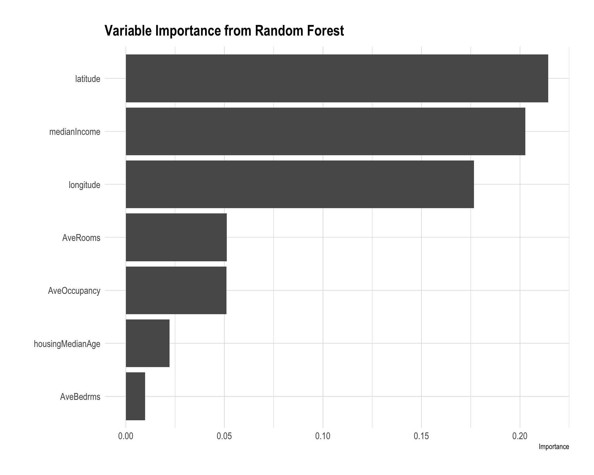
The random forest model averages predictions across many regression trees, which usually improves predictive accuracy relative to a single tree by reducing variance.
The variable importance plot shows that latitude, median income, and longitude are the most important predictors. This suggests that both location and income level play major roles in predicting median housing value. Other housing characteristics, such as average rooms, average occupancy, housing median age, and average bedrooms, are less important in this model.
partial(rf_fit, pred.var = "medianIncome", train = dtrain) |>
  autoplot() +
  labs(title = "Partial Dependence of Housing Price on medianIncome")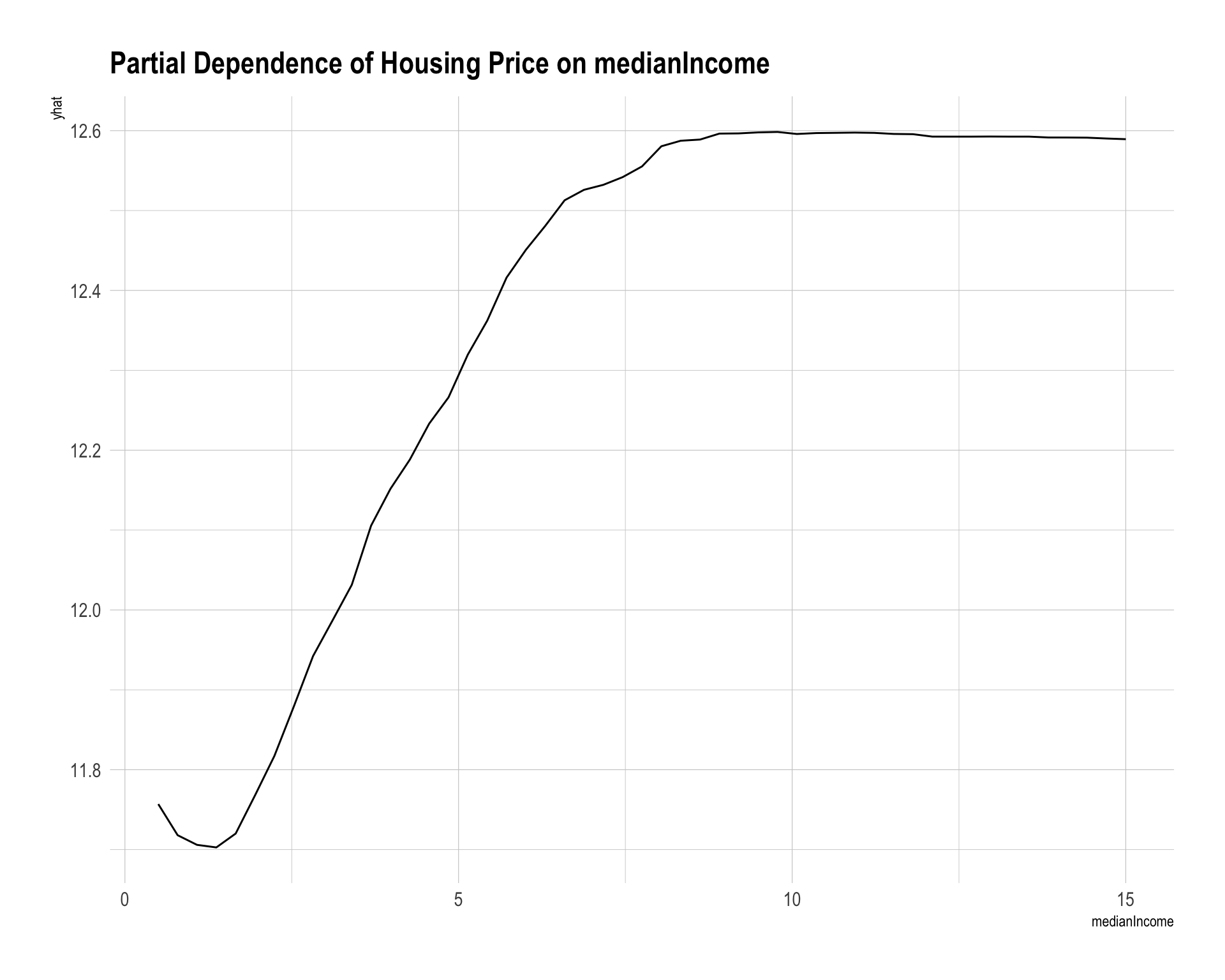
Question 9
Fit a gradient-boosted tree model using the following hyperparameter grid:
xgb_grid <- tidyr::crossing(
  nrounds = seq(20, 200, by = 20),
  eta = c(0.025, 0.05, 0.1, 0.3),
  max_depth = c(2, 3),
  gamma = c(0),
  colsample_bytree = c(1),
  min_child_weight = c(1),
  subsample = c(1)
)

xgb_grid |>
  paged_table()
Show answer
set.seed(42120532)

x_train_mat <- dtrain |>
  select(housingMedianAge, medianIncome, AveBedrms, AveRooms, AveOccupancy,
         latitude, longitude) |>
  as.matrix()

x_test_mat <- dtest |>
  select(housingMedianAge, medianIncome, AveBedrms, AveRooms, AveOccupancy,
         latitude, longitude) |>
  as.matrix()

dMat_train <- xgb.DMatrix(data = x_train_mat, label = y_train)

xgb_results_lst <- vector("list", nrow(xgb_grid))

for (i in seq_len(nrow(xgb_grid))) {
  nrounds <- xgb_grid$nrounds[i]
  eta <- xgb_grid$eta[i]
  max_depth <- xgb_grid$max_depth[i]
  gamma <- xgb_grid$gamma[i]
  colsample_bytree <- xgb_grid$colsample_bytree[i]
  min_child_weight <- xgb_grid$min_child_weight[i]
  subsample <- xgb_grid$subsample[i]

  cv_fit <- xgb.cv(
    data = dMat_train,
    nrounds = nrounds,
    nfold = 5,
    objective = "reg:squarederror",
    eta = eta,
    max_depth = max_depth,
    gamma = gamma,
    colsample_bytree = colsample_bytree,
    min_child_weight = min_child_weight,
    subsample = subsample,
    verbose = 0
  )

  xgb_results_lst[[i]] <- tibble(
    nrounds = nrounds,
    eta = eta,
    max_depth = max_depth,
    gamma = gamma,
    colsample_bytree = colsample_bytree,
    min_child_weight = min_child_weight,
    subsample = subsample,
    cv_rmse = min(cv_fit$evaluation_log$test_rmse_mean)
  )
}

xgb_results <- bind_rows(xgb_results_lst) |>
  arrange(cv_rmse)

xgb_results |>
  paged_table()
best_xgb <- xgb_results |>
slice_min(cv_rmse, n = 1)
best_xgb |>
paged_table()set.seed(42120532)
xgb_fit_final <- xgboost(
data = x_train_mat,
label = y_train,
objective = "reg:squarederror",
nrounds = best_xgb$nrounds,
eta = best_xgb$eta,
max_depth = best_xgb$max_depth,
gamma = best_xgb$gamma,
colsample_bytree = best_xgb$colsample_bytree,
min_child_weight = best_xgb$min_child_weight,
subsample = best_xgb$subsample,
verbose = 0
)
xgb_fit_finalXGBoost model object
Call:
xgboost(objective = "reg:squarederror", nrounds = best_xgb$nrounds,
max_depth = best_xgb$max_depth, min_child_weight = best_xgb$min_child_weight,
subsample = best_xgb$subsample, colsample_bytree = best_xgb$colsample_bytree,
data = x_train_mat, label = y_train, eta = best_xgb$eta,
gamma = best_xgb$gamma, verbose = 0)
Objective: reg:squarederror
Number of iterations: 200
Number of features: 7The gradient-boosted tree model builds trees sequentially. Each new tree attempts to improve on the errors of the previous trees. The cross-validation process chooses the combination of tuning parameters with the best validation performance.
vip(xgb_fit_final) +
  labs(title = "XGBoost Variable Importance")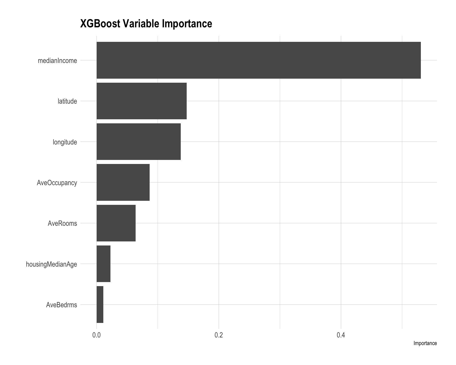
partial(
  xgb_fit_final,
  pred.var = "medianIncome",
  train = x_train_mat,
  plot = TRUE,
  plot.engine = "ggplot2",
  type = "regression"
) +
  labs(title = "XGBoost Partial Dependence of Housing Price on medianIncome")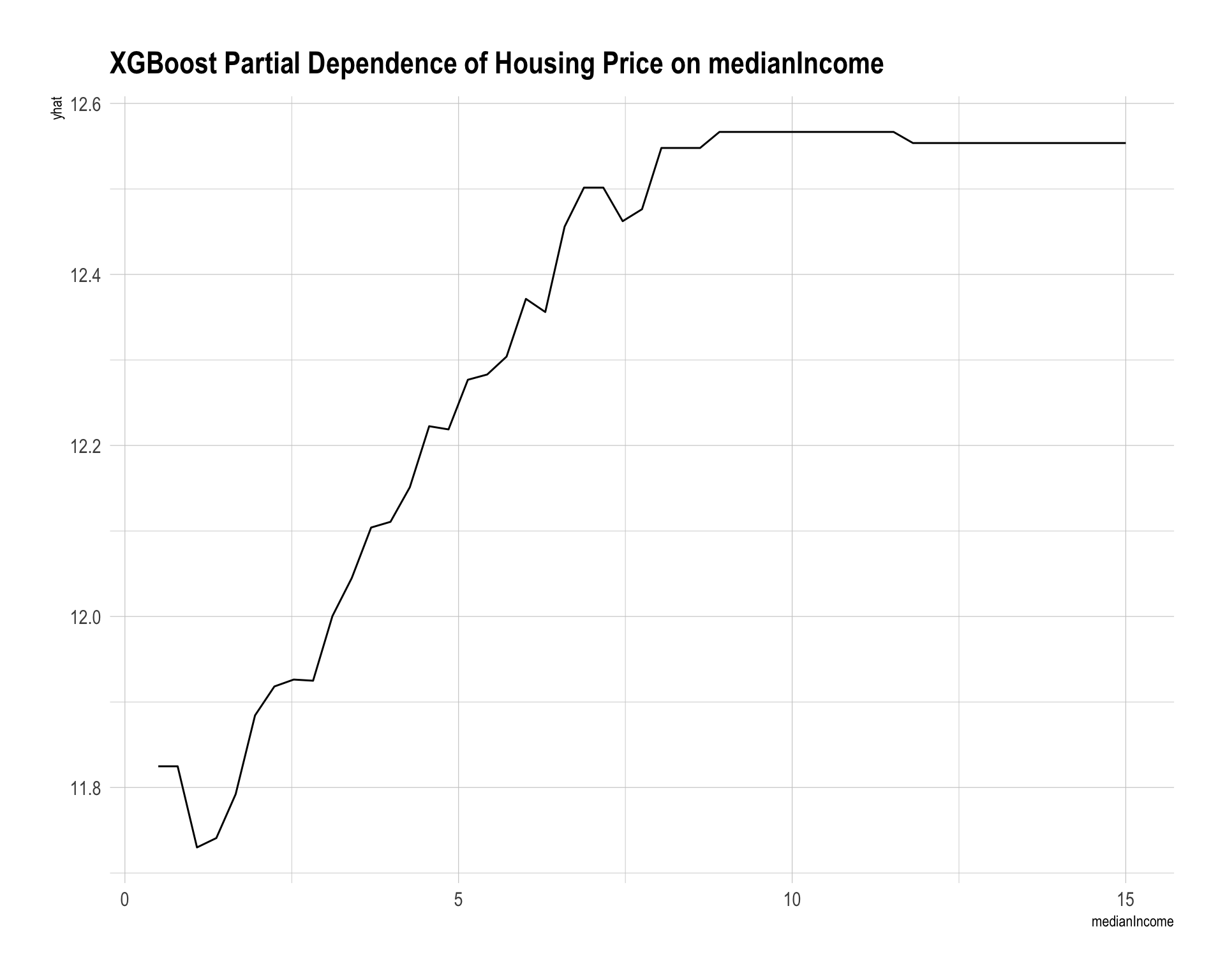
Question 10
Compare the prediction performance across the models:
- Linear regression
- Lasso regression
- Ridge regression
- Regression tree
- Random forest
- Gradient-boosted tree
Show answer
pred_lm_test <- predict(lm_fit, newdata = dtest)
pred_lasso_test <- as.numeric(predict(lasso_fit, newx = x_test, s = "lambda.min"))
pred_ridge_test <- as.numeric(predict(ridge_fit, newx = x_test, s = "lambda.min"))
pred_tree_test <- predict(tree_fit, newdata = dtest)
pred_rf_test <- predict(rf_fit, data = dtest)$predictions
pred_xgb_test <- predict(xgb_fit_final, newdata = dtest)
model_performance <- tibble(
model = c(
"Linear regression",
"Lasso regression",
"Ridge regression",
"Regression tree",
"Random forest",
"Gradient-boosted tree"
),
rmse = c(
sqrt(mean((y_test - pred_lm_test)^2)),
sqrt(mean((y_test - pred_lasso_test)^2)),
sqrt(mean((y_test - pred_ridge_test)^2)),
sqrt(mean((y_test - pred_tree_test)^2)),
sqrt(mean((y_test - pred_rf_test)^2)),
sqrt(mean((y_test - pred_xgb_test)^2))
),
mae = c(
mean(abs(y_test - pred_lm_test)),
mean(abs(y_test - pred_lasso_test)),
mean(abs(y_test - pred_ridge_test)),
mean(abs(y_test - pred_tree_test)),
mean(abs(y_test - pred_rf_test)),
mean(abs(y_test - pred_xgb_test))
)
) |>
arrange(rmse)
model_performance |>
mutate(
rmse = round(rmse, 4),
mae = round(mae, 4)
) |>
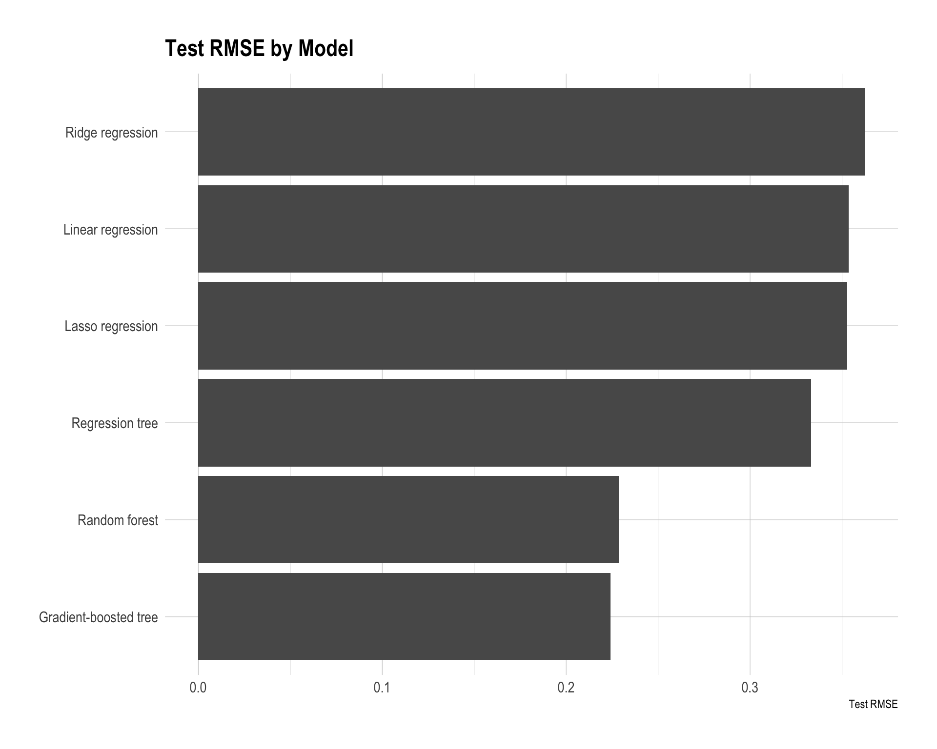
paged_table()model_performance |>
ggplot(aes(x = reorder(model, rmse), y = rmse)) +
geom_col() +
coord_flip() +
labs(
title = "Test RMSE by Model",
x = NULL,
y = "Test RMSE"
)
resid_df <- tibble(
actual = y_test,
`Linear regression` = pred_lm_test,
`Lasso regression` = pred_lasso_test,
`Ridge regression` = pred_ridge_test,
`Regression tree` = pred_tree_test,
`Random forest` = pred_rf_test,
`Gradient-boosted tree` = pred_xgb_test
) |>
pivot_longer(
cols = -actual,
names_to = "model",
values_to = "prediction"
) |>
mutate(abs_error = abs(actual - prediction))
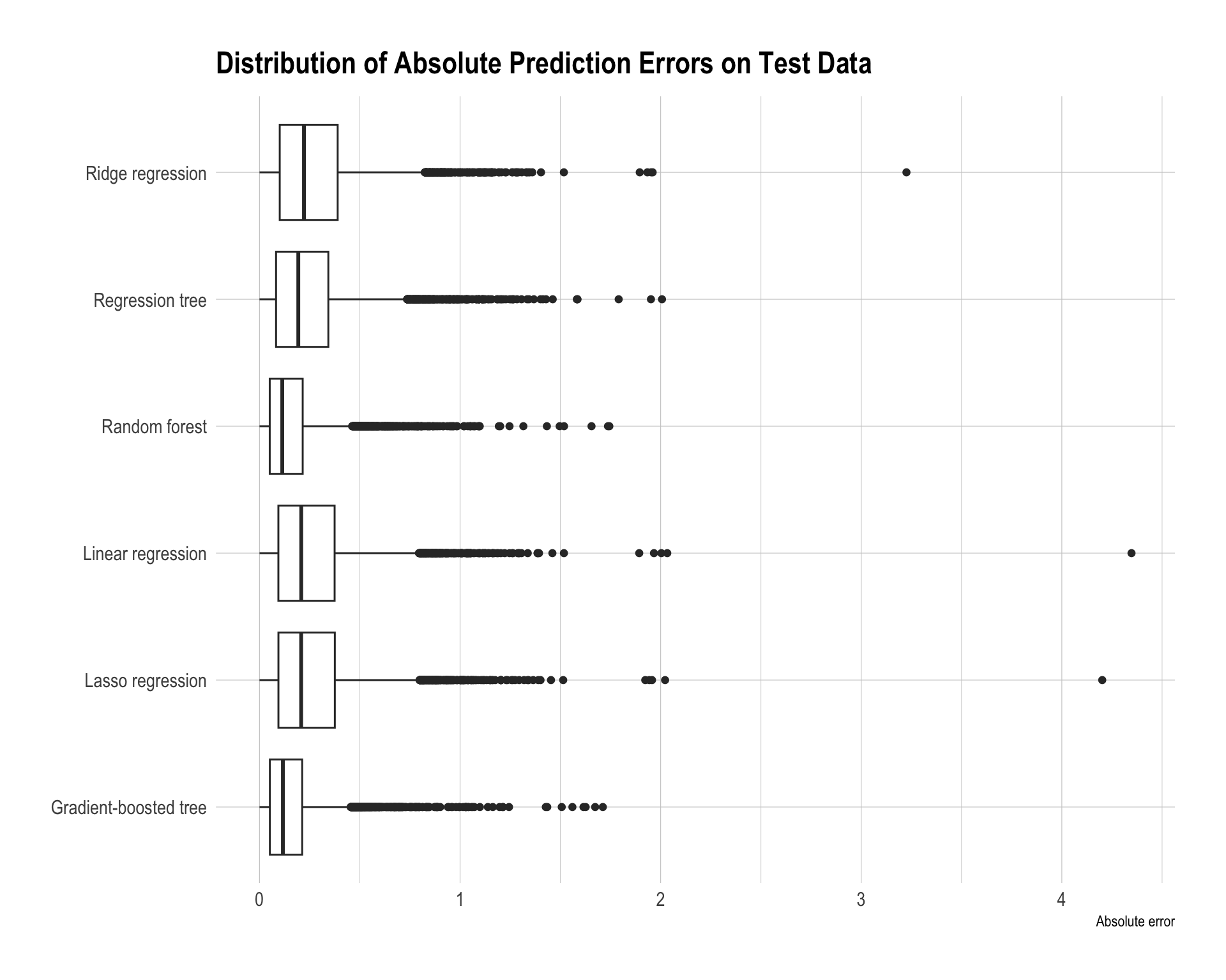
resid_df |>
ggplot(aes(x = model, y = abs_error)) +
geom_boxplot() +
coord_flip() +
labs(
title = "Distribution of Absolute Prediction Errors on Test Data",
x = NULL,
y = "Absolute error"
)
The best model is the gradient-boosted tree, as it achieves the smallest test RMSE (0.2240) and also the lowest MAE. The random forest performs very similarly with an RMSE of 0.2287, indicating that tree-based ensemble methods clearly outperform the other models in this task.
The regression tree improves over the linear models but still has noticeably higher error, with an RMSE of about 0.3117. This suggests that a single tree is not flexible enough compared with ensemble methods.
The linear-based models — linear regression, lasso regression, and ridge regression — perform the worst, with RMSE values around 0.35–0.36. This suggests that the relationship between predictors such as income, housing characteristics, location, and housing prices is likely nonlinear and may involve interactions that linear models cannot capture well, even with regularization.
Overall, the results show that ensemble tree methods, especially gradient boosting, provide the best predictive performance because they can effectively model nonlinear patterns and complex interactions in the data.
library(ggmap)
library(ggthemes)

google_api <- "YOUR_GOOGLE_MAP_API_KEY"

register_google(google_api)

ca_map <- get_map(location = "California", zoom = 6)

CA.test.map.agg <- dtest |>
  mutate(
    Actual = exp(y_test),
    `Linear regression` = exp(pred_lm_test),
    `Lasso regression` = exp(pred_lasso_test),
    `Ridge regression` = exp(pred_ridge_test),
    `Regression tree` = exp(pred_tree_test),
    `Random forest` = exp(pred_rf_test),
    `Gradient-boosted tree` = exp(pred_xgb_test)
  ) |>
  select(
    longitude,
    latitude,
    Actual,
    `Linear regression`,
    `Lasso regression`,
    `Ridge regression`,
    `Regression tree`,
    `Random forest`,
    `Gradient-boosted tree`
  ) |>
  group_by(longitude, latitude) |>
  summarise(
    across(where(is.numeric), \(x) mean(x, na.rm = TRUE)),
    .groups = "drop"
  )

CA_error_vis <- dtest |>
  mutate(
    actual = exp(y_test),
    `Linear regression` = exp(pred_lm_test),
    `Lasso regression` = exp(pred_lasso_test),
    `Ridge regression` = exp(pred_ridge_test),
    `Regression tree` = exp(pred_tree_test),
    `Random forest` = exp(pred_rf_test),
    `Gradient-boosted tree` = exp(pred_xgb_test)
  ) |>
  pivot_longer(
    cols = c(
      `Linear regression`,
      `Lasso regression`,
      `Ridge regression`,
      `Regression tree`,
      `Random forest`,
      `Gradient-boosted tree`
    ),
    names_to = "model",
    values_to = "prediction"
  ) |>
  mutate(
    error = prediction - actual,
    model = factor(model,
                   levels = c(
                     "Linear regression",
                     "Lasso regression",
                     "Ridge regression",
                     "Regression tree",
                     "Random forest",
                     "Gradient-boosted tree"
                   ),
                   labels = c(
                     "Linear regression",
                     "Lasso regression",
                     "Ridge regression",
                     "Regression tree",
                     "Random forest",
                     "Gradient-boosted tree"
                   ))
  )

error_limit <- quantile(abs(CA_error_vis$error), 0.98, na.rm = TRUE)

ggmap(ca_map) +
  geom_point(
    data = CA_error_vis,
    aes(x = longitude, y = latitude, color = error),
    size = 0.55,
    alpha = 0.55
  ) +
  scale_color_gradient2(
    name = "Prediction\nerror ($)",
    low = "#005AB5",      # underprediction: strong blue
    mid = "#F7F7F7",      # near-perfect prediction: light/white
    high = "#DC3220",     # overprediction: strong red
    midpoint = 0,
    limits = c(-error_limit, error_limit),
    oob = squish,
    trans = pseudo_log_trans(sigma = 10000),
    breaks = c(
      -200000, -100000, -50000, -25000,
      0,
      25000, 50000, 100000, 200000
    ),
    labels = function(x) format(round(x), big.mark = ",", scientific = FALSE),
    na.value = "grey50"
  ) +
  facet_wrap(~ model, ncol = 2) +
  labs(
    title = "Prediction Errors in California Housing Values",
    subtitle = "Blue = underprediction; white = close prediction; red = overprediction",
    x = NULL,
    y = NULL
  ) +
  theme_map() +
  theme(
    legend.position = "right",
    strip.text = element_text(face = "bold")
  ) +
  guides(
    color = guide_colorbar(
      direction = "vertical",
      barheight = 68,
      title.position = "top"
    )
  )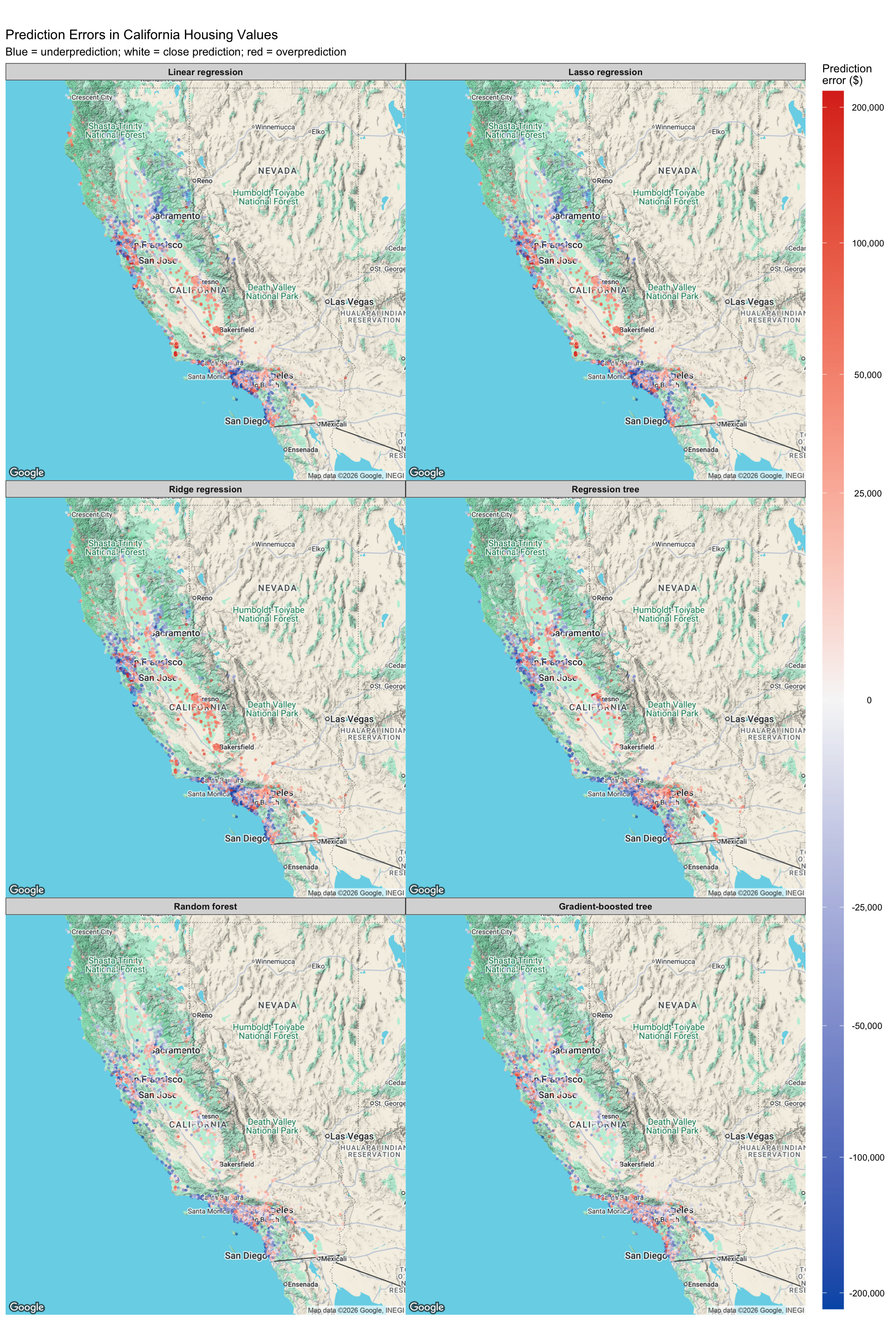
The error maps show where each model tends to make larger prediction errors. In the maps, red points indicate overprediction, blue points indicate underprediction, and white or light-colored points indicate predictions close to the actual value.
The linear regression, lasso regression, and ridge regression models show very similar spatial error patterns. They tend to underpredict high-value coastal areas, especially around the Bay Area, Los Angeles, Orange County, and parts of the San Diego area. They also show some overprediction in inland areas, including parts of the Central Valley. This suggests that linear models have difficulty capturing strong nonlinear location effects in California housing prices.
The regression tree reduces some of the linear-model error patterns but still produces noticeable regional errors. Because a single tree makes predictions using a limited number of split-based regions, it may be too coarse to fully capture smooth variation in housing prices across space.
The random forest and gradient-boosted tree maps show less extreme and less systematic error patterns. They still make some errors in expensive coastal markets, but the errors are more balanced across regions. This supports the test RMSE results, where the ensemble tree models perform better than the single tree and the linear models.
Overall, the map suggests that location is one of the most important drivers of prediction error. The best models are the ones that better capture nonlinear spatial patterns and interactions between location, income, and housing characteristics.