library(tidyverse)
library(broom)
library(stargazer)

library(glmnet)
library(gamlr)
library(Matrix)

library(DT)
library(rmarkdown)
library(hrbrthemes)
library(ggthemes)

theme_set(
  theme_ipsum()
)

scale_colour_discrete <- function(...) scale_color_colorblind(...)
scale_fill_discrete <- function(...) scale_fill_colorblind(...)Homework 3
Lasso Linear Regression
Direction
Please submit one Quarto Document of Homework 3 to Brightspace using the following file naming convention:
Example:
danl-320-hw3-choe-byeonghak.qmd
Due: March 9, 2026, 11:59 P.M. (ET)
Please send Byeong-Hak an email (
bchoe@geneseo.edu) if you have any questions.
Consider the beer_markets data.frame from Homework 1:
beer_markets <- read_csv(
  'https://bcdanl.github.io/data/beer_markets_all_cleaned.csv'
) |>
  select(-region, -state) |>   # removing region and state variables
  filter(container %in% c("CAN", "NON_REFILLABLE_BOTTLE")) |>
  mutate(logprice = log(price_floz)) |>
  mutate(across(where(is.character), as.factor))    # convert all character columns to factors
Variable Description
| Variable Name | Description |
|---|---|
household |
Unique identifier for household |
X_purchase_desc |
Description of beer purchase |
quantity |
Number of beer packages purchased |
brand |
Brand of beer purchased |
dollar_spent |
Total amount spent on the purchase |
beer_floz |
Total volume of beer purchased (in fluid ounces) |
price_floz |
Price per fluid ounce of beer |
container |
Type of beer container (e.g., CAN, BOTTLE) |
promo |
Indicates if the purchase was part of a promotion (True/False) |
market |
Market region of purchase |
marital |
Marital status of household head |
income |
Income level of the household |
age |
Age group of household head |
employment |
Employment status of household head |
degree |
Education level of household head |
occupation |
Occupation category of household head |
ethnic |
Ethnicity of household head |
microwave |
Indicates if the household owns a microwave (True/False) |
dishwasher |
Indicates if the household owns a dishwasher (True/False) |
tvcable |
Type of television subscription (e.g., basic, premium) |
singlefamilyhome |
Indicates if the household is a single-family home (True/False) |
npeople |
Number of people in the household |
Data Preparation
# Setting a missing value (NA) as a reference level of a factor
xnaref <- function(x){
  if(is.factor(x))
    if(!is.na(levels(x)[1]))
      x <- factor(x,levels=c(NA,levels(x)),exclude=NULL)
  return(x) }

naref <- function(DF){
  if(is.null(dim(DF))) return(xnaref(DF))
  if(!is.data.frame(DF))
    stop("You need to give me a data.frame or a factor")
  DF <- lapply(DF, xnaref)
  return(as.data.frame(DF))
}

beer_markets_naref <- naref(beer_markets)

# Checking unique values of factor variable, brand
unique(beer_markets$brand)
[1] BUD_LIGHT BUSCH_LIGHT COORS_LIGHT MILLER_LITE NATURAL_LIGHT
Levels: BUD_LIGHT BUSCH_LIGHT COORS_LIGHT MILLER_LITE NATURAL_LIGHTunique(beer_markets_naref$brand)[1] BUD_LIGHT BUSCH_LIGHT COORS_LIGHT MILLER_LITE NATURAL_LIGHT
Levels: <NA> BUD_LIGHT BUSCH_LIGHT COORS_LIGHT MILLER_LITE NATURAL_LIGHT# Checking levels of factor variable, brand
levels(beer_markets_naref$brand) [1] NA "BUD_LIGHT" "BUSCH_LIGHT" "COORS_LIGHT"
[5] "MILLER_LITE" "NATURAL_LIGHT"levels(beer_markets$brand) [1] "BUD_LIGHT" "BUSCH_LIGHT" "COORS_LIGHT" "MILLER_LITE"
[5] "NATURAL_LIGHT"Training and Test Sets
# 1) reproducible split
set.seed(1)  # you can choose any seed

# 2) sample row indices
beer_markets_naref <- beer_markets_naref |>
  mutate(rnd = runif(n())) # n() number of random numbers from Unif(0,1) are drawn

# 2-1) sample row indices for training (about 67%)
dtrain <- beer_markets_naref |>
  filter(rnd >= 0.33) |>
  select(-rnd)

# 2-1) sample row indices for test (about 33%)
dtest <- beer_markets_naref |>
  filter(rnd < 0.33) |>
  select(-rnd)
Linear Regression Models
Regular Model 1
\[ \begin{aligned} \log(\text{dollar\_spent}) = &\ \beta_{0} + \sum_{i=1}^{N} \beta_{i} \,\text{market}_{i} + \sum_{j=N+1}^{N+4} \beta_{j} \,\text{brand}_{j} + \beta_{N+5} \,\text{container\_CAN} \\ &\,+\, \beta_{N+6} \log(\text{price\_floz}) + \epsilon \end{aligned} \]
Regular Model 2 (brand-specific price sensitivity)
\[ \begin{aligned} \log(\text{dollar\_spent}) \,=\, & \beta_{0} + \sum_{i=1}^{N}\beta_{i}\,\text{market}_{i} \,+\, \sum_{j=N+1}^{N+4}\beta_{j}\,\text{brand}_{j} \,+\, \beta_{N+5}\,\text{container\_CAN} \\ &\,+\, \beta_{N+6}\log(\text{price\_floz})\\ &\,+\, \sum_{j=N+1}^{N+4}\beta_{j\times\text{price\_floz}}\,\text{brand}_{j}\times \log(\text{price\_floz})\\ &\,+\, \epsilon \end{aligned} \]
Regular Model 3 (promo + brand-specific promo effects)
\[ \begin{aligned} \log(\text{dollar\_spent}) \,=\, & \beta_{0} + \sum_{i=1}^{N}\beta_{i}\,\text{market}_{i} \,+\, \sum_{j=N+1}^{N+4}\beta_{j}\,\text{brand}_{j} \,+\, \beta_{N+5}\,\text{container\_CAN} \\ &\,+\, \beta_{N+6}\log(\text{price\_floz})\\ &\,+\, \beta_{N+7}\,\text{promo} \times\log(\text{price\_floz}) \\ &\,+\, \sum_{j=N+1}^{N+4}\beta_{j\times\text{price\_floz}}\,\text{brand}_{j}\times \log(\text{price\_floz})\\ &\,+\, \sum_{j=N+1}^{N+4}\beta_{j\times\text{promo}}\,\text{brand}_{j}\times \text{promo}\\ &\,+\, \sum_{j=N+1}^{N+4}\beta_{j\times\text{promo}\times\text{price\_floz}}\,\text{brand}_{j}\times \text{promo}\times \log(\text{price\_floz})\\ &\,+\, \epsilon \end{aligned} \]
Lasso Linear Regression Models
Sparse Matrices for a Bigger Demographics Design
Building a sparse matrix for a bigger demographics design by interacting with market
- Demographics matrix (
Xdemog): Interactsmarketwith all demographic variables, capturing how the effect of each demographic characteristic varies across markets- Dataset
Xdemogin Details:- Individual Demographic Dummies: As described previously.
- Interaction Terms: Constructed by interacting the
marketdummies with each of the demographic dummies from thebeer_marketsdata.frame
- Dataset
- Beer matrix (
Xbeer): Captureslogpriceandbrandmain effects - Beer \(\times\) Brand matrix (
Xbeer_brand): Two-way interaction betweenlogpriceandbrand— allowing price elasticity to differ by brand - Beer \(\times\) Brand \(\times\) Promo matrix (
Xbeer_brand_promo): Full three-way interaction amonglogprice,brand, andpromo— allowing price elasticity to differ by brand and promotional status
All matrices are stored as sparse matrices to save memory, since most market \(\times\) demographic combinations are zero.
# Building a sparse matrix for a bigger demographics design
# by interacting with market

Xdemog_train <- model.matrix(
  ~ market * (buyertype + income + childrenUnder6 + children6to17 +
                age + employment + degree + occupation + ethnic +
                microwave + dishwasher + tvcable + singlefamilyhome +
                npeople),
  data=dtrain)[,-1] |>
  Matrix(sparse = TRUE)   # converting it to a sparse matrix

Xdemog_test <- model.matrix(
  ~ market * (buyertype + income + childrenUnder6 + children6to17 +
                age + employment + degree + occupation + ethnic +
                microwave + dishwasher + tvcable + singlefamilyhome +
                npeople),
  data=dtest)[,-1] |>
  Matrix(sparse = TRUE)   # converting it to a sparse matrix

Xbeer_train <- model.matrix(
  ~ logprice + brand + container,
  data=dtrain)[,-1] |>
  Matrix(sparse = TRUE)
Xbeer_test <- model.matrix(
  ~ logprice + brand + container,
  data=dtest)[,-1] |>
  Matrix(sparse = TRUE)

Xbeer_brand_train <- model.matrix(
  ~ logprice * brand + container,
  data=dtrain)[,-1] |>
  Matrix(sparse = TRUE)
Xbeer_brand_test <- model.matrix(
  ~ logprice * brand + container,
  data=dtest)[,-1] |>
  Matrix(sparse = TRUE)

Xbeer_brand_promo_train <- model.matrix(
  ~ logprice * brand * promo + container,
  data=dtrain)[,-1] |>
  Matrix(sparse = TRUE)
Xbeer_brand_promo_test <- model.matrix(
  ~ logprice * brand * promo + container,
  data=dtest)[,-1] |>
  Matrix(sparse = TRUE)

y_train <- log(dtrain$dollar_spent)
y_test <- log(dtest$dollar_spent)rm(beer_markets, beer_markets_naref)\[ \begin{align} &\text{market}\\ &\text{marital}\\ &\text{age}\\ &\text{employment}\\ &\text{degree}\\ &\text{occupation}\\ &\text{ethnic}\\ &\text{microwave}\\ &\text{dishwasher}\\ &\text{tvcable}\\ &\text{singlefamilyhome}\\ &\text{npeople} \end{align} \]
\[ \begin{align} &\text{market}\times \text{marital}\\ &\text{market}\times \text{income}\\ &\text{market}\times \text{age}\\ &\text{market}\times \text{employment}\\ &\text{market}\times \text{degree}\\ &\text{market}\times \text{occupation}\\ &\text{market}\times \text{ethnic}\\ &\text{market}\times \text{microwave}\\ &\text{market}\times \text{dishwasher}\\ &\text{market}\times \text{tvcable}\\ &\text{market}\times \text{singlefamilyhome}\\ &\text{market}\times \text{npeople} \end{align} \]
Models
The three models below extend those from the above linear regression models by replacing the separate market dummies with the full Xdemog matrix — adding market × demographic interactions.
Lasso Model 1
\[ \begin{aligned} \log(\text{dollar\_spent}) \,=\, & \sum_{j=1}^{4} \beta_{j}\,\text{brand}_{j} \,+\, \beta_{5}\,\text{container\_CAN} \\ &\,+\, \beta_{6}\log(\text{price\_floz})\\ &\,+\, \sum_{k=7}^{K}\beta_{k}\,\text{demographics}_{k}\\ &\,+\, \epsilon \end{aligned} \]
where \(\text{demographics}_{k}\) refers to all columns in Xdemog (individual market/demographic dummies and their interactions).
Lasso Model 2 (brand-specific volume sensitivity)
\[ \begin{aligned} \log(\text{dollar\_spent}) \,=\, & \sum_{j=1}^{4}\beta_{j}\,\text{brand}_{j} \,+\, \beta_{5}\,\text{container\_CAN} \\ &\,+\, \beta_{6}\log(\text{price\_floz})\\ &\,+\, \sum_{j=1}^{4}\beta_{j\times\text{price\_floz}}\,\text{brand}_{j}\times \log(\text{price\_floz})\\ &\,+\, \sum_{k=7}^{K}\beta_{k}\,\text{demographics}_{k}\\ &\,+\, \epsilon \end{aligned} \]
Lasso Model 3 (promo + brand-specific promo effects)
\[ \begin{aligned} \log(\text{dollar\_spent}) \,=\, & \sum_{j=1}^{4}\beta_{j}\,\text{brand}_{j} \,+\, \beta_{5}\,\text{container\_CAN} \\ &\,+\, \beta_{6}\log(\text{price\_floz})\\ &\,+\, \beta_{7}\,\text{promo} \times\log(\text{price\_floz}) \\ &\,+\, \sum_{j=1}^{4}\beta_{j\times\text{price\_floz}}\,\text{brand}_{j}\times \log(\text{price\_floz})\\ &\,+\, \sum_{j=1}^{4}\beta_{j\times\text{promo}}\,\text{brand}_{j}\times \text{promo}\\ &\,+\, \sum_{j=1}^{4}\beta_{j\times\text{promo}\times\text{price\_floz}}\,\text{brand}_{j}\times \text{promo}\times \log(\text{price\_floz})\\ &\,+\, \sum_{k=7}^{K}\beta_{k}\,\text{demographics}_{k}\\ &\,+\, \epsilon \end{aligned} \]
- With this large demographic design, Lasso Model 3 includes 3,695 predictors.
- This count excludes the all-zero (empty) columns that would otherwise arise from some market \(\times\) demographic interaction terms.
❓ Questions
Question 1 — Estimate models
- Fit all models.
- Determine the optimal value of the lambda parameter for each Lasso model.
For Lasso models, use cbind() to bind matrices into one input matrix:
cbind(Xbeer_train, Xdemog_train)   # Lasso Model 1
cbind(Xbeer_brand_train, Xdemog_train)   # Lasso Model 2
cbind(Xbeer_brand_promo_train, Xdemog_train)   # Lasso Model 3
Show answer
Dummy Variables, Reference Coding, and the Intercept in Regularized Regression
For factor (categorical) predictors, you have two clean choices.
Option A: K−1 dummies and keep the intercept
Use model.matrix() with R’s default reference-category coding (drops one level as the reference), and remove the intercept column before passing x to glmnet.
- Interpretation (K−1 dummies): each dummy coefficient is the effect of that category relative to the reference level.
Option B: K dummies but remove the intercept
Keep all \(K\) dummy columns (no reference category), and set intercept = FALSE.
Then collinearity disappears, and each \(\beta_k\) acts like the category’s “absolute level”.
- Interpretation (K dummies): each category coefficient \(\beta_k\) is the category’s baseline contribution.
In this homework, we choose Option B: K dummies but remove the intercept.
Fitting the Models
m1 <- lm(data = dtrain,
         log(dollar_spent) ~ logprice + brand + container + market)
m2 <- lm(data = dtrain,
         log(dollar_spent) ~ logprice * brand + container + market)
m3 <- lm(data = dtrain,
         log(dollar_spent) ~ logprice * brand * promo + container + market)

model_1 <- cv.glmnet(cbind(Xbeer_train, Xdemog_train), y_train,
                     alpha     = 1,
                     intercept = FALSE   # TRUE is default
                     )

model_2 <- cv.glmnet(cbind(Xbeer_brand_train, Xdemog_train), y_train,
                     alpha     = 1,
                     intercept = FALSE   # TRUE is default
                     )

model_3 <- cv.glmnet(cbind(Xbeer_brand_promo_train, Xdemog_train), y_train,
                     alpha     = 1,
                     intercept = FALSE   # TRUE is default
                     )

model_1_int <- cv.glmnet(cbind(Xbeer_train, Xdemog_train), y_train,
                         alpha     = 1
                         )

model_2_int <- cv.glmnet(cbind(Xbeer_brand_train, Xdemog_train), y_train,
                         alpha     = 1
                         )

model_3_int <- cv.glmnet(cbind(Xbeer_brand_promo_train, Xdemog_train), y_train,
                         alpha     = 1
                         )
\(\lambda\)
lambdas_1 <- model_1 |>
  glance()

lambdas_2 <- model_2 |>
  glance()

lambdas_3 <- model_3 |>
  glance()

lambdas_1_int <- model_1_int |>
  glance()

lambdas_2_int <- model_2_int |>
  glance()

lambdas_3_int <- model_3_int |>
  glance()

lambdas_all <- rbind(
  lambdas_1 |> mutate(model = "Lasso Model 1 without Intercept", .before = 0),
  lambdas_2 |> mutate(model = "Lasso Model 2 without Intercept", .before = 0),
  lambdas_3 |> mutate(model = "Lasso Model 3 without Intercept", .before = 0),
  lambdas_1_int |> mutate(model = "Lasso Model 1 with Intercept", .before = 0),
  lambdas_2_int |> mutate(model = "Lasso Model 2 with Intercept", .before = 0),
  lambdas_3_int |> mutate(model = "Lasso Model 3 with Intercept", .before = 0)
)

lambdas_all |>
  paged_table()
Question 2 — Price sensitivity and promo (elasticities)
- Across the six models in this homework, how is the percentage change in the beer expenditure sensitive to the percentage change in the price of beer for each brand?
- How does incorporating a broader demographic design into the model affect this?
Show answer
Betas
# Regular Models
m1_beta <- m1 |>
  tidy(conf.int = T) |>
  mutate(
    stars = case_when(
      p.value < .01 ~ "***",  # smallest p-values first
      p.value < .05 ~ "**",
      p.value < .1 ~ "*",
      TRUE ~ ""
    ),
    .after = estimate
  ) |>
  select(term, estimate, stars, starts_with("conf")) |>
  mutate(model = "Regular Model 1",
         .before = 1)

m2_beta <- m2 |>
  tidy(conf.int = T) |>
  mutate(
    stars = case_when(
      p.value < .01 ~ "***",  # smallest p-values first
      p.value < .05 ~ "**",
      p.value < .1 ~ "*",
      TRUE ~ ""
    ),
    .after = estimate
  ) |>
  select(term, estimate, stars, starts_with("conf")) |>
  mutate(model = "Regular Model 2",
         .before = 1)

m3_beta <- m3 |>
  tidy(conf.int = T) |>
  mutate(
    stars = case_when(
      p.value < .01 ~ "***",  # smallest p-values first
      p.value < .05 ~ "**",
      p.value < .1 ~ "*",
      TRUE ~ ""
    ),
    .after = estimate
  ) |>
  select(term, estimate, stars, starts_with("conf")) |>
  mutate(model = "Regular Model 3",
         .before = 1)


betas_linear <- bind_rows(m1_beta, m2_beta, m3_beta) |>
  arrange(term, model)


# Lasso Models
## Lasso Models without Intercept
model_1_beta_1se <- coef(model_1,
                         s = "lambda.1se")  # default
model_1_beta_min <- coef(model_1,
                         s = "lambda.min")

model_2_beta_1se <- coef(model_2,
                         s = "lambda.1se")  # default
model_2_beta_min <- coef(model_2,
                         s = "lambda.min")

model_3_beta_1se <- coef(model_3,
                         s = "lambda.1se")  # default
model_3_beta_min <- coef(model_3,
                         s = "lambda.min")

## Lasso Models with Intercept
model_1_int_beta_1se <- coef(model_1_int,
                             s = "lambda.1se")  # default
model_1_int_beta_min <- coef(model_1_int,
                             s = "lambda.min")

model_2_int_beta_1se <- coef(model_2_int,
                             s = "lambda.1se")  # default
model_2_int_beta_min <- coef(model_2_int,
                             s = "lambda.min")

model_3_int_beta_1se <- coef(model_3_int,
                             s = "lambda.1se")  # default
model_3_int_beta_min <- coef(model_3_int,
                             s = "lambda.min")


betas_model_1 <- data.frame(
  term = rownames(model_1_beta_1se),
  beta_lasso_1se = as.numeric(model_1_beta_1se),
  beta_lasso_min = as.numeric(model_1_beta_min)
) |>
  mutate(model = "Lasso Model 1 without Intercept",
         .before = 1)


betas_model_2 <- data.frame(
  term = rownames(model_2_beta_1se),
  beta_lasso_1se = as.numeric(model_2_beta_1se),
  beta_lasso_min = as.numeric(model_2_beta_min)
) |>
  mutate(model = "Lasso Model 2 without Intercept",
         .before = 1)


betas_model_3 <- data.frame(
  term = rownames(model_3_beta_1se),
  beta_lasso_1se = as.numeric(model_3_beta_1se),
  beta_lasso_min = as.numeric(model_3_beta_min)
) |>
  mutate(model = "Lasso Model 3 without Intercept",
         .before = 1)


betas_model_1_int <- data.frame(
  term = rownames(model_1_int_beta_1se),
  beta_lasso_1se = as.numeric(model_1_int_beta_1se),
  beta_lasso_min = as.numeric(model_1_int_beta_min)
) |>
  mutate(model = "Lasso Model 1 with Intercept",
         .before = 1)


betas_model_2_int <- data.frame(
  term = rownames(model_2_int_beta_1se),
  beta_lasso_1se = as.numeric(model_2_int_beta_1se),
  beta_lasso_min = as.numeric(model_2_int_beta_min)
) |>
  mutate(model = "Lasso Model 2 with Intercept",
         .before = 1)


betas_model_3_int <- data.frame(
  term = rownames(model_3_int_beta_1se),
  beta_lasso_1se = as.numeric(model_3_int_beta_1se),
  beta_lasso_min = as.numeric(model_3_int_beta_min)
) |>
  mutate(model = "Lasso Model 3 with Intercept",
         .before = 1)

betas_lasso <- bind_rows(
  betas_model_1, betas_model_2, betas_model_3,
  betas_model_1_int, betas_model_2_int, betas_model_3_int
)

# Long-form data.frame
betas_lasso_long <- betas_lasso |>
  pivot_longer(cols = beta_lasso_1se:beta_lasso_min,
               names_to = "lambda",
               values_to = "beta") |>
  mutate(lambda = str_replace(lambda,
                              "beta_lasso_", ""))

betas_linear_stars <- betas_linear |>
  filter(stars != "") |>
  rename(beta = estimate) |>
  select(model, term, beta) |>
  mutate(lambda = "0",
         .after = term)

betas_all <- bind_rows(betas_linear_stars,
                       betas_lasso_long)

betas_all |>
  paged_table()
Betas for Elasticities
betas_elasticity <- betas_all |>
  filter(str_detect(term, "logprice")) |>
  arrange(model, term, lambda)

betas_elasticity |>
  paged_table()
Summary of Price Elasticities using coef()
Since we use all dummies in a predictor matrix, we should consider Lasso models without an intercept.
elas_1se_bud <- data.frame(
  Model = c("Regular 1",
            "Regular 2",
            "Regular 3",
            "Lasso 1 with Intercept",
            "Lasso 1 without Intercept",
            "Lasso 2 with Intercept",
            "Lasso 2 without Intercept",
            "Lasso 3 with Intercept",
            "Lasso 3 without Intercept"),
  Bud = c(
    coef(m1)['logprice'],
    coef(m2)['logprice'],
    coef(m3)['logprice'],
    coef(model_1_int)['logprice', ],
    coef(model_1)['logprice', ],
    coef(model_2_int)['logprice', ] + coef(model_2_int)['logprice:brandBUD_LIGHT', ],
    coef(model_2)['logprice', ] + coef(model_2)['logprice:brandBUD_LIGHT', ],
    coef(model_3_int)['logprice', ] + coef(model_3_int)['logprice:brandBUD_LIGHT', ],
    coef(model_3)['logprice', ] + coef(model_3)['logprice:brandBUD_LIGHT', ]
  ),
  Bud_promo = c(
    NA,
    NA,
    coef(m3)['logprice'] + coef(m3)['logprice:promoTRUE'],
    NA,
    NA,
    NA,
    NA,
    coef(model_3_int)['logprice', ] + coef(model_3_int)['logprice:brandBUD_LIGHT', ]
      + coef(model_3_int)['logprice:brandBUD_LIGHT:promoTRUE', ] + coef(model_3_int)['logprice:brandBUD_LIGHT:promoTRUE', ],
    coef(model_3)['logprice', ] + coef(model_3)['logprice:brandBUD_LIGHT', ]
      + coef(model_3)['logprice:brandBUD_LIGHT:promoTRUE', ] + coef(model_3)['logprice:brandBUD_LIGHT:promoTRUE', ]
  )
)


elas_1se_busch <- data.frame(
  Model = c("Regular 1",
            "Regular 2",
            "Regular 3",
            "Lasso 1 with Intercept",
            "Lasso 1 without Intercept",
            "Lasso 2 with Intercept",
            "Lasso 2 without Intercept",
            "Lasso 3 with Intercept",
            "Lasso 3 without Intercept"),
  Busch = c(
    coef(m1)['logprice'],
    coef(m2)['logprice'],  #  coef(m2)['logprice:brandBUSCH_LIGHT'] is not stat. sig.
    coef(m3)['logprice'] + coef(m3)['logprice:brandBUSCH_LIGHT'],
    coef(model_1_int)['logprice', ],
    coef(model_1)['logprice', ],
    coef(model_2_int)['logprice', ] + coef(model_2_int)['logprice:brandBUSCH_LIGHT', ],
    coef(model_2)['logprice', ] + coef(model_2)['logprice:brandBUSCH_LIGHT', ],
    coef(model_3_int)['logprice', ] + coef(model_3_int)['logprice:brandBUSCH_LIGHT', ],
    coef(model_3)['logprice', ] + coef(model_3)['logprice:brandBUSCH_LIGHT', ]
  ),
  Busch_promo = c(
    NA,
    NA,
    coef(m3)['logprice'] + coef(m3)['logprice:promoTRUE']
    + coef(m3)['logprice:brandBUSCH_LIGHT'] + coef(m3)['logprice:brandBUSCH_LIGHT:promoTRUE'],
    NA,
    NA,
    NA,
    NA,
    coef(model_3_int)['logprice', ] + coef(model_3_int)['logprice:brandBUSCH_LIGHT', ]
    + coef(model_3_int)['logprice:brandBUSCH_LIGHT:promoTRUE', ] + coef(model_3_int)['logprice:brandBUSCH_LIGHT:promoTRUE', ],
    coef(model_3)['logprice', ] + coef(model_3)['logprice:brandBUSCH_LIGHT', ]
    + coef(model_3)['logprice:brandBUSCH_LIGHT:promoTRUE', ] + coef(model_3)['logprice:brandBUSCH_LIGHT:promoTRUE', ]
  )
)


elas_1se_coors <- data.frame(
  Model = c("Regular 1",
            "Regular 2",
            "Regular 3",
            "Lasso 1 with Intercept",
            "Lasso 1 without Intercept",
            "Lasso 2 with Intercept",
            "Lasso 2 without Intercept",
            "Lasso 3 with Intercept",
            "Lasso 3 without Intercept"),
  Coors = c(
    coef(m1)['logprice'],
    coef(m2)['logprice'] + coef(m2)['logprice:brandCOORS_LIGHT'],
    coef(m3)['logprice'] + coef(m3)['logprice:brandCOORS_LIGHT'],
    coef(model_1_int)['logprice', ],
    coef(model_1)['logprice', ],
    coef(model_2_int)['logprice', ] + coef(model_2_int)['logprice:brandCOORS_LIGHT', ],
    coef(model_2)['logprice', ] + coef(model_2)['logprice:brandCOORS_LIGHT', ],
    coef(model_3_int)['logprice', ] + coef(model_3_int)['logprice:brandCOORS_LIGHT', ],
    coef(model_3)['logprice', ] + coef(model_3)['logprice:brandCOORS_LIGHT', ]
  ),
  Coors_promo = c(
    NA,
    NA,
    coef(m3)['logprice'] + coef(m3)['logprice:promoTRUE']
    + coef(m3)['logprice:brandCOORS_LIGHT'] + coef(m3)['logprice:brandCOORS_LIGHT:promoTRUE'],
    NA,
    NA,
    NA,
    NA,
    coef(model_3_int)['logprice', ] + coef(model_3_int)['logprice:brandCOORS_LIGHT', ]
    + coef(model_3_int)['logprice:brandCOORS_LIGHT:promoTRUE', ] + coef(model_3_int)['logprice:brandCOORS_LIGHT:promoTRUE', ],
    coef(model_3)['logprice', ] + coef(model_3)['logprice:brandCOORS_LIGHT', ]
    + coef(model_3)['logprice:brandCOORS_LIGHT:promoTRUE', ] + coef(model_3)['logprice:brandCOORS_LIGHT:promoTRUE', ]
  )
)

elas_1se_miller <- data.frame(
  Model = c("Regular 1",
            "Regular 2",
            "Regular 3",
            "Lasso 1 with Intercept",
            "Lasso 1 without Intercept",
            "Lasso 2 with Intercept",
            "Lasso 2 without Intercept",
            "Lasso 3 with Intercept",
            "Lasso 3 without Intercept"),
  Miller = c(
    coef(m1)['logprice'],
    coef(m2)['logprice'] + coef(m2)['logprice:brandMILLER_LITE'],
    coef(m3)['logprice'] + coef(m3)['logprice:brandMILLER_LITE'],
    coef(model_1_int)['logprice', ],
    coef(model_1)['logprice', ],
    coef(model_2_int)['logprice', ] + coef(model_2_int)['logprice:brandMILLER_LITE', ],
    coef(model_2)['logprice', ] + coef(model_2)['logprice:brandMILLER_LITE', ],
    coef(model_3_int)['logprice', ] + coef(model_3_int)['logprice:brandMILLER_LITE', ],
    coef(model_3)['logprice', ] + coef(model_3)['logprice:brandMILLER_LITE', ]
  ),
  Miller_promo = c(
    NA,
    NA,
    coef(m3)['logprice'] + coef(m3)['logprice:promoTRUE']
    + coef(m3)['logprice:brandMILLER_LITE'] ,  # coef(m3)['logprice:brandMILLER_LITE:promoTRUE'] is not stat. sig.
    NA,
    NA,
    NA,
    NA,
    coef(model_3_int)['logprice', ] + coef(model_3_int)['logprice:brandMILLER_LITE', ]
    + coef(model_3_int)['logprice:brandMILLER_LITE:promoTRUE', ] + coef(model_3_int)['logprice:brandMILLER_LITE:promoTRUE', ],
    coef(model_3)['logprice', ] + coef(model_3)['logprice:brandMILLER_LITE', ]
    + coef(model_3)['logprice:brandMILLER_LITE:promoTRUE', ] + coef(model_3)['logprice:brandMILLER_LITE:promoTRUE', ]
  )
)

elas_1se_natural <- data.frame(
  Model = c("Regular 1",
            "Regular 2",
            "Regular 3",
            "Lasso 1 with Intercept",
            "Lasso 1 without Intercept",
            "Lasso 2 with Intercept",
            "Lasso 2 without Intercept",
            "Lasso 3 with Intercept",
            "Lasso 3 without Intercept"),
  Natural = c(
    coef(m1)['logprice'],
    coef(m2)['logprice'] + coef(m2)['logprice:brandNATURAL_LIGHT'],
    coef(m3)['logprice'] + coef(m3)['logprice:brandNATURAL_LIGHT'],
    coef(model_1_int)['logprice', ],
    coef(model_1)['logprice', ],
    coef(model_2_int)['logprice', ] + coef(model_2_int)['logprice:brandNATURAL_LIGHT', ],
    coef(model_2)['logprice', ] + coef(model_2)['logprice:brandNATURAL_LIGHT', ],
    coef(model_3_int)['logprice', ] + coef(model_3_int)['logprice:brandNATURAL_LIGHT', ],
    coef(model_3)['logprice', ] + coef(model_3)['logprice:brandNATURAL_LIGHT', ]
  ),
  Natural_promo = c(
    NA,
    NA,
    coef(m3)['logprice'] + coef(m3)['logprice:promoTRUE']
    + coef(m3)['logprice:brandNATURAL_LIGHT'] + coef(m3)['logprice:brandNATURAL_LIGHT:promoTRUE'],
    NA,
    NA,
    NA,
    NA,
    coef(model_3_int)['logprice', ] + coef(model_3_int)['logprice:brandNATURAL_LIGHT', ]
    + coef(model_3_int)['logprice:brandNATURAL_LIGHT:promoTRUE', ] + coef(model_3_int)['logprice:brandNATURAL_LIGHT:promoTRUE', ],
    coef(model_3)['logprice', ] + coef(model_3)['logprice:brandNATURAL_LIGHT', ]
    + coef(model_3)['logprice:brandNATURAL_LIGHT:promoTRUE', ] + coef(model_3)['logprice:brandNATURAL_LIGHT:promoTRUE', ]
  )
)

elas_1se_all <- elas_1se_bud |>
  left_join(elas_1se_busch) |>
  left_join(elas_1se_coors) |>
  left_join(elas_1se_miller) |>
  left_join(elas_1se_natural)
elas_min_bud <- data.frame(
Model = c("Regular 1",
"Regular 2",
"Regular 3",
"Lasso 1 with Intercept",
"Lasso 1 without Intercept",
"Lasso 2 with Intercept",
"Lasso 2 without Intercept",
"Lasso 3 with Intercept",
"Lasso 3 without Intercept"),
Bud = c(
coef(m1)['logprice'],
coef(m2)['logprice'],
coef(m3)['logprice'],
coef(model_1_int, s = 'lambda.min')['logprice', ],
coef(model_1, s = 'lambda.min')['logprice', ],
coef(model_2_int, s = 'lambda.min')['logprice', ] + coef(model_2_int, s = 'lambda.min')['logprice:brandBUD_LIGHT', ],
coef(model_2, s = 'lambda.min')['logprice', ] + coef(model_2, s = 'lambda.min')['logprice:brandBUD_LIGHT', ],
coef(model_3_int, s = 'lambda.min')['logprice', ] + coef(model_3_int, s = 'lambda.min')['logprice:brandBUD_LIGHT', ],
coef(model_3, s = 'lambda.min')['logprice', ] + coef(model_3, s = 'lambda.min')['logprice:brandBUD_LIGHT', ]
),
Bud_promo = c(
NA,
NA,
coef(m3)['logprice'] + coef(m3)['logprice:promoTRUE'],
NA,
NA,
NA,
NA,
coef(model_3_int, s = 'lambda.min')['logprice', ] + coef(model_3_int, s = 'lambda.min')['logprice:brandBUD_LIGHT', ]
+ coef(model_3_int, s = 'lambda.min')['logprice:brandBUD_LIGHT:promoTRUE', ] + coef(model_3_int, s = 'lambda.min')['logprice:brandBUD_LIGHT:promoTRUE', ],
coef(model_3, s = 'lambda.min')['logprice', ] + coef(model_3, s = 'lambda.min')['logprice:brandBUD_LIGHT', ]
+ coef(model_3, s = 'lambda.min')['logprice:brandBUD_LIGHT:promoTRUE', ] + coef(model_3, s = 'lambda.min')['logprice:brandBUD_LIGHT:promoTRUE', ]
)
)
elas_min_busch <- data.frame(
Model = c("Regular 1",
"Regular 2",
"Regular 3",
"Lasso 1 with Intercept",
"Lasso 1 without Intercept",
"Lasso 2 with Intercept",
"Lasso 2 without Intercept",
"Lasso 3 with Intercept",
"Lasso 3 without Intercept"),
Busch = c(
coef(m1)['logprice'],
coef(m2)['logprice'], # coef(m2)['logprice:brandBUSCH_LIGHT'] is not stat. sig.
coef(m3)['logprice'] + coef(m3)['logprice:brandBUSCH_LIGHT'],
coef(model_1_int, s = 'lambda.min')['logprice', ],
coef(model_1, s = 'lambda.min')['logprice', ],
coef(model_2_int, s = 'lambda.min')['logprice', ] + coef(model_2_int, s = 'lambda.min')['logprice:brandBUSCH_LIGHT', ],
coef(model_2, s = 'lambda.min')['logprice', ] + coef(model_2, s = 'lambda.min')['logprice:brandBUSCH_LIGHT', ],
coef(model_3_int, s = 'lambda.min')['logprice', ] + coef(model_3_int, s = 'lambda.min')['logprice:brandBUSCH_LIGHT', ],
coef(model_3, s = 'lambda.min')['logprice', ] + coef(model_3, s = 'lambda.min')['logprice:brandBUSCH_LIGHT', ]
),
Busch_promo = c(
NA,
NA,
coef(m3)['logprice'] + coef(m3)['logprice:promoTRUE']
+ coef(m3)['logprice:brandBUSCH_LIGHT'] + coef(m3)['logprice:brandBUSCH_LIGHT:promoTRUE'],
NA,
NA,
NA,
NA,
coef(model_3_int, s = 'lambda.min')['logprice', ] + coef(model_3_int, s = 'lambda.min')['logprice:brandBUSCH_LIGHT', ]
+ coef(model_3_int, s = 'lambda.min')['logprice:brandBUSCH_LIGHT:promoTRUE', ] + coef(model_3_int, s = 'lambda.min')['logprice:brandBUSCH_LIGHT:promoTRUE', ],
coef(model_3, s = 'lambda.min')['logprice', ] + coef(model_3, s = 'lambda.min')['logprice:brandBUSCH_LIGHT', ]
+ coef(model_3, s = 'lambda.min')['logprice:brandBUSCH_LIGHT:promoTRUE', ] + coef(model_3, s = 'lambda.min')['logprice:brandBUSCH_LIGHT:promoTRUE', ]
)
)
elas_min_coors <- data.frame(
Model = c("Regular 1",
"Regular 2",
"Regular 3",
"Lasso 1 with Intercept",
"Lasso 1 without Intercept",
"Lasso 2 with Intercept",
"Lasso 2 without Intercept",
"Lasso 3 with Intercept",
"Lasso 3 without Intercept"),
Coors = c(
coef(m1)['logprice'],
coef(m2)['logprice'] + coef(m2)['logprice:brandCOORS_LIGHT'],
coef(m3)['logprice'] + coef(m3)['logprice:brandCOORS_LIGHT'],
coef(model_1_int, s = 'lambda.min')['logprice', ],
coef(model_1, s = 'lambda.min')['logprice', ],
coef(model_2_int, s = 'lambda.min')['logprice', ] + coef(model_2_int, s = 'lambda.min')['logprice:brandCOORS_LIGHT', ],
coef(model_2, s = 'lambda.min')['logprice', ] + coef(model_2, s = 'lambda.min')['logprice:brandCOORS_LIGHT', ],
coef(model_3_int, s = 'lambda.min')['logprice', ] + coef(model_3_int, s = 'lambda.min')['logprice:brandCOORS_LIGHT', ],
coef(model_3, s = 'lambda.min')['logprice', ] + coef(model_3, s = 'lambda.min')['logprice:brandCOORS_LIGHT', ]
),
Coors_promo = c(
NA,
NA,
coef(m3)['logprice'] + coef(m3)['logprice:promoTRUE']
+ coef(m3)['logprice:brandCOORS_LIGHT'] + coef(m3)['logprice:brandCOORS_LIGHT:promoTRUE'],
NA,
NA,
NA,
NA,
coef(model_3_int, s = 'lambda.min')['logprice', ] + coef(model_3_int, s = 'lambda.min')['logprice:brandCOORS_LIGHT', ]
+ coef(model_3_int, s = 'lambda.min')['logprice:brandCOORS_LIGHT:promoTRUE', ] + coef(model_3_int, s = 'lambda.min')['logprice:brandCOORS_LIGHT:promoTRUE', ],
coef(model_3, s = 'lambda.min')['logprice', ] + coef(model_3, s = 'lambda.min')['logprice:brandCOORS_LIGHT', ]
+ coef(model_3, s = 'lambda.min')['logprice:brandCOORS_LIGHT:promoTRUE', ] + coef(model_3, s = 'lambda.min')['logprice:brandCOORS_LIGHT:promoTRUE', ]
)
)
elas_min_miller <- data.frame(
Model = c("Regular 1",
"Regular 2",
"Regular 3",
"Lasso 1 with Intercept",
"Lasso 1 without Intercept",
"Lasso 2 with Intercept",
"Lasso 2 without Intercept",
"Lasso 3 with Intercept",
"Lasso 3 without Intercept"),
Miller = c(
coef(m1)['logprice'],
coef(m2)['logprice'] + coef(m2)['logprice:brandMILLER_LITE'],
coef(m3)['logprice'] + coef(m3)['logprice:brandMILLER_LITE'],
coef(model_1_int, s = 'lambda.min')['logprice', ],
coef(model_1, s = 'lambda.min')['logprice', ],
coef(model_2_int, s = 'lambda.min')['logprice', ] + coef(model_2_int, s = 'lambda.min')['logprice:brandMILLER_LITE', ],
coef(model_2, s = 'lambda.min')['logprice', ] + coef(model_2, s = 'lambda.min')['logprice:brandMILLER_LITE', ],
coef(model_3_int, s = 'lambda.min')['logprice', ] + coef(model_3_int, s = 'lambda.min')['logprice:brandMILLER_LITE', ],
coef(model_3, s = 'lambda.min')['logprice', ] + coef(model_3, s = 'lambda.min')['logprice:brandMILLER_LITE', ]
),
Miller_promo = c(
NA,
NA,
coef(m3)['logprice'] + coef(m3)['logprice:promoTRUE']
+ coef(m3)['logprice:brandMILLER_LITE'] , # coef(m3)['logprice:brandMILLER_LITE:promoTRUE'] is not stat. sig.
NA,
NA,
NA,
NA,
coef(model_3_int, s = 'lambda.min')['logprice', ] + coef(model_3_int, s = 'lambda.min')['logprice:brandMILLER_LITE', ]
+ coef(model_3_int, s = 'lambda.min')['logprice:brandMILLER_LITE:promoTRUE', ] + coef(model_3_int, s = 'lambda.min')['logprice:brandMILLER_LITE:promoTRUE', ],
coef(model_3, s = 'lambda.min')['logprice', ] + coef(model_3, s = 'lambda.min')['logprice:brandMILLER_LITE', ]
+ coef(model_3, s = 'lambda.min')['logprice:brandMILLER_LITE:promoTRUE', ] + coef(model_3, s = 'lambda.min')['logprice:brandMILLER_LITE:promoTRUE', ]
)
)
elas_min_natural <- data.frame(
Model = c("Regular 1",
"Regular 2",
"Regular 3",
"Lasso 1 with Intercept",
"Lasso 1 without Intercept",
"Lasso 2 with Intercept",
"Lasso 2 without Intercept",
"Lasso 3 with Intercept",
"Lasso 3 without Intercept"),
Natural = c(
coef(m1)['logprice'],
coef(m2)['logprice'] + coef(m2)['logprice:brandNATURAL_LIGHT'],
coef(m3)['logprice'] + coef(m3)['logprice:brandNATURAL_LIGHT'],
coef(model_1_int, s = 'lambda.min')['logprice', ],
coef(model_1, s = 'lambda.min')['logprice', ],
coef(model_2_int, s = 'lambda.min')['logprice', ] + coef(model_2_int, s = 'lambda.min')['logprice:brandNATURAL_LIGHT', ],
coef(model_2, s = 'lambda.min')['logprice', ] + coef(model_2, s = 'lambda.min')['logprice:brandNATURAL_LIGHT', ],
coef(model_3_int, s = 'lambda.min')['logprice', ] + coef(model_3_int, s = 'lambda.min')['logprice:brandNATURAL_LIGHT', ],
coef(model_3, s = 'lambda.min')['logprice', ] + coef(model_3, s = 'lambda.min')['logprice:brandNATURAL_LIGHT', ]
),
Natural_promo = c(
NA,
NA,
coef(m3)['logprice'] + coef(m3)['logprice:promoTRUE']
+ coef(m3)['logprice:brandNATURAL_LIGHT'] + coef(m3)['logprice:brandNATURAL_LIGHT:promoTRUE'],
NA,
NA,
NA,
NA,
coef(model_3_int, s = 'lambda.min')['logprice', ] + coef(model_3_int, s = 'lambda.min')['logprice:brandNATURAL_LIGHT', ]
+ coef(model_3_int, s = 'lambda.min')['logprice:brandNATURAL_LIGHT:promoTRUE', ] + coef(model_3_int, s = 'lambda.min')['logprice:brandNATURAL_LIGHT:promoTRUE', ],
coef(model_3, s = 'lambda.min')['logprice', ] + coef(model_3, s = 'lambda.min')['logprice:brandNATURAL_LIGHT', ]
+ coef(model_3, s = 'lambda.min')['logprice:brandNATURAL_LIGHT:promoTRUE', ] + coef(model_3, s = 'lambda.min')['logprice:brandNATURAL_LIGHT:promoTRUE', ]
)
)
elas_min_all <- elas_min_bud |>
left_join(elas_min_busch) |>
left_join(elas_min_coors) |>
left_join(elas_min_miller) |>
left_join(elas_min_natural)elas_min_all_tmp <- elas_min_all |>
filter(str_detect(Model, "Lasso")) |>
filter(str_detect(Model, "without ")) |>
mutate(Model = str_replace(Model,
"without Intercept",
"without Intercept (lambda.min)"))
elas_all <- elas_1se_all |>
filter(!str_detect(Model, "with ")) |>
bind_rows(elas_min_all_tmp) |>
arrange(Model)
elas_all |>
select(Model:Busch_promo) |>
paged_table()elas_all |>
select(Model, Coors:Miller_promo) |>
paged_table()elas_all |>
select(Model, Natural:Natural_promo) |>
paged_table()Across all three models, beer expenditure is price elastic for every brand: the estimated elasticities are negative, meaning a higher price is associated with lower beer expenditure for that brand. In the \(\lambda_{1se}\) lasso results, Bud/Busch/Coors/Miller cluster tightly around about \(-0.63\) to \(-0.65\), while Natural Light is less sensitive at about \(-0.49\) to \(-0.50\) (smaller magnitude).
With a richer demographic specification, the model can better capture heterogeneity in spending patterns (different baseline expenditure levels across demographic segments), so the brand price coefficients reflect a cleaner price response rather than absorbing demographic-driven differences. In the results, this shows up as moving from a near “one common elasticity” pattern (Model 1) to more brand-specific elasticities (Models 2–3), especially highlighting that Natural Light demand is less price-sensitive than the other brands.
🧾 Interpreting the elasticity table
Each number in the table is a (log-log) price elasticity estimate: - Example: \(\beta = -0.64\) means a 1% increase in price is associated with about a 0.64% decrease in beer expenditure, holding the other included variables fixed.
A more negative elasticity (e.g., \(-1.99\)) implies more price-sensitive beer expenditure.
0) Regular (unpenalized) models: much larger magnitudes (likely inflated / unstable)
- Regular 1: all brands \(-1.65\)
- Regular 2: around \(-1.63\) to \(-1.74\)
- Regular 3: as negative as \(-1.99\), plus promo elasticities like \(-0.79\), \(-1.46\), etc.
Interpretation
- These are much larger in magnitude than the lasso estimates (about 2–3× larger).
- This often happens when the unpenalized model suffers from multicollinearity or too many regressors, which inflates coefficient magnitudes and variance.
- In elasticity work, that’s a classic reason to prefer penalized estimates (especially \(\lambda_{1se}\)) when the main goal is a stable elasticity rather than best in-sample fit.
1) Lasso 1 (without intercept): all brands have the same elasticity
- Bud = Busch = Coors = Miller = Natural \(\approx -0.635\)
Interpretation
- Model 1 is imposing a strong restriction: the data are being fit as if all brands share one common price elasticity, and promo effects are not modeled.
- Lasso shrinkage makes that shared estimate very stable: about \(-0.64\).
2) Lasso 2 (without intercept): elasticities vary by brand (Natural is less elastic)
- Bud / Coors / Miller \(\approx -0.65\)
- Busch \(\approx -0.64\)
- Natural \(\approx -0.50\)
Interpretation
- This specification allows more flexibility than Model 1.
- The key pattern: Natural has a smaller magnitude elasticity (less negative), meaning its demand is less price-sensitive than the other brands in this model.
3) Lasso 3 (without intercept): promo effects enter, but are “tied” to base effects in several cases
Many are very close to their corresponding base elasticity:
Bud: \(\beta_{\text{price}} \approx -0.638\), \(\beta_{\text{promo}} \approx -0.638\)
Similar equality appears for Busch and Coors, and for Miller both are about \(-0.638\)
Natural: price \(\approx -0.495\), promo \(\approx -0.484\)
In Model 3, promo effects are being estimated, but the model is telling you the promo terms are not separately identifiable.
Promo effect may be:
- weak once brand and other covariates are included,
- unstable across CV folds (e.g., useful in some folds but not others),
- or relevant only for one segment/brand (Natural Light).
So at both \(\lambda_{1se}\) and \(\lambda_{\min}\), lasso shrinks the promo coefficients to exactly \(0\) because, after controlling for price and the other covariates, including promo does not reduce cross-validated prediction error enough to “earn” a nonzero coefficient. In other words, across the CV folds the promo variables either add only a tiny improvement, add an improvement that appears in some folds but not others, or add information that is already captured by existing predictors, so the lasso penalty treats them as not worth keeping and sets them to \(0\).
- Also, Natural Light promotion has the strongest incremental signal in data, while other promo terms are too small/noisy to survive.
Question 3 — Predict and evaluate
- Using the test dataset, compare the root Mean Squared Errors (RMSEs) across models.
For Lasso models, use cbind() to bind matrices into one input matrix:
cbind(Xbeer_test, Xdemog_test)   # Lasso Model 1
cbind(Xbeer_brand_test, Xdemog_test)   # Lasso Model 2
cbind(Xbeer_brand_promo_test, Xdemog_test)   # Lasso Model 3
Show answer
pred_linear <- dtest |>
  mutate(pred_1 = predict(m1, newdata = dtest),
         pred_2 = predict(m2, newdata = dtest),
         pred_3 = predict(m3, newdata = dtest),
         resid_1 = log(dollar_spent) - pred_1,
         resid_2 = log(dollar_spent) - pred_2,
         resid_3 = log(dollar_spent) - pred_3
         ) |>
  select(dollar_spent, pred_1:resid_3)

RMSEs_linear <- pred_linear |>
  mutate(
    resid_1_sq = resid_1^2,
    resid_2_sq = resid_2^2,
    resid_3_sq = resid_3^2
  ) |>
  summarize(
    RMSE_1_linear = sqrt( mean(resid_1_sq) ),
    RMSE_2_linear = sqrt( mean(resid_2_sq) ),
    RMSE_3_linear = sqrt( mean(resid_3_sq) )
  )
pred_lasso <- dtest |>
mutate(
.fitted_m1_lasso_1se = predict(model_1, newx = cbind(Xbeer_test, Xdemog_test),
s = "lambda.1se"),
.fitted_m1_lasso_min = predict(model_1, newx = cbind(Xbeer_test, Xdemog_test),
s = "lambda.min"),
.fitted_m2_lasso_1se = predict(model_2, newx = cbind(Xbeer_brand_test, Xdemog_test),
s = "lambda.1se"),
.fitted_m2_lasso_min = predict(model_2, newx = cbind(Xbeer_brand_test, Xdemog_test),
s = "lambda.min"),
.fitted_m3_lasso_1se = predict(model_3, newx = cbind(Xbeer_brand_promo_test, Xdemog_test),
s = "lambda.1se"),
.fitted_m3_lasso_min = predict(model_3, newx = cbind(Xbeer_brand_promo_test, Xdemog_test),
s = "lambda.min"),
.resid_m1_lasso_1se = log(dollar_spent) - .fitted_m1_lasso_1se,
.resid_m1_lasso_min = log(dollar_spent) - .fitted_m1_lasso_min,
.resid_m2_lasso_1se = log(dollar_spent) - .fitted_m2_lasso_1se,
.resid_m2_lasso_min = log(dollar_spent) - .fitted_m2_lasso_min,
.resid_m3_lasso_1se = log(dollar_spent) - .fitted_m3_lasso_1se,
.resid_m3_lasso_min = log(dollar_spent) - .fitted_m3_lasso_min
) |>
select(dollar_spent, .fitted_m1_lasso_1se:.resid_m3_lasso_min)
RMSEs_lasso <- pred_lasso |>
mutate(
.resid_m1_lasso_1se_sq = .resid_m1_lasso_1se^2,
.resid_m1_lasso_min_sq = .resid_m1_lasso_min^2,
.resid_m2_lasso_1se_sq = .resid_m2_lasso_1se^2,
.resid_m2_lasso_min_sq = .resid_m2_lasso_min^2,
.resid_m3_lasso_1se_sq = .resid_m3_lasso_1se^2,
.resid_m3_lasso_min_sq = .resid_m3_lasso_min^2
) |>
summarise(
RMSE_m1_lasso_1se = sqrt( mean(.resid_m1_lasso_1se_sq) ),
RMSE_m1_lasso_min = sqrt( mean(.resid_m1_lasso_min_sq) ),
RMSE_m2_lasso_1se = sqrt( mean(.resid_m2_lasso_1se_sq) ),
RMSE_m2_lasso_min = sqrt( mean(.resid_m2_lasso_min_sq) ),
RMSE_m3_lasso_1se = sqrt( mean(.resid_m3_lasso_1se_sq) ),
RMSE_m3_lasso_min = sqrt( mean(.resid_m3_lasso_min_sq) )
) RMSE_all <- bind_cols(RMSEs_linear, RMSEs_lasso) |>
t() |>
as.data.frame() |>
rename(RMSE = V1)
RMSE_all$Model <- str_replace(rownames(RMSE_all), "RMSE_", "")
rownames(RMSE_all) <- 1:nrow(RMSE_all)
RMSE_all <- RMSE_all |>
relocate(Model) |>
arrange(RMSE)
RMSE_all |>
paged_table()- All Lasso models (
model_1–model_3) perform somewhat better than the unregularized linear models (m1–m3), but the difference does not appear dramatic.- Lasso RMSE is about 0.51, while the linear models have RMSE about 0.575.
- This suggests the unregularized models may be somewhat less stable out of sample, possibly due to many predictors or multicollinearity.
- Differences among Lasso models are tiny.
- The best RMSE is m3_lasso_min = 0.5072, but the other lasso models are extremely close (within about 0.003).
- Practically, these lasso models have very similar predictive performance.
Question 4 — Choose a preferred model
Which model do you prefer most and why? Your answer must reference at least two of the following:
- out-of-sample performance (test RMSE)
- interpretability / simplicity
- whether interactions and bigger demographic designs are substantively meaningful
- residual plot patterns
Show answer
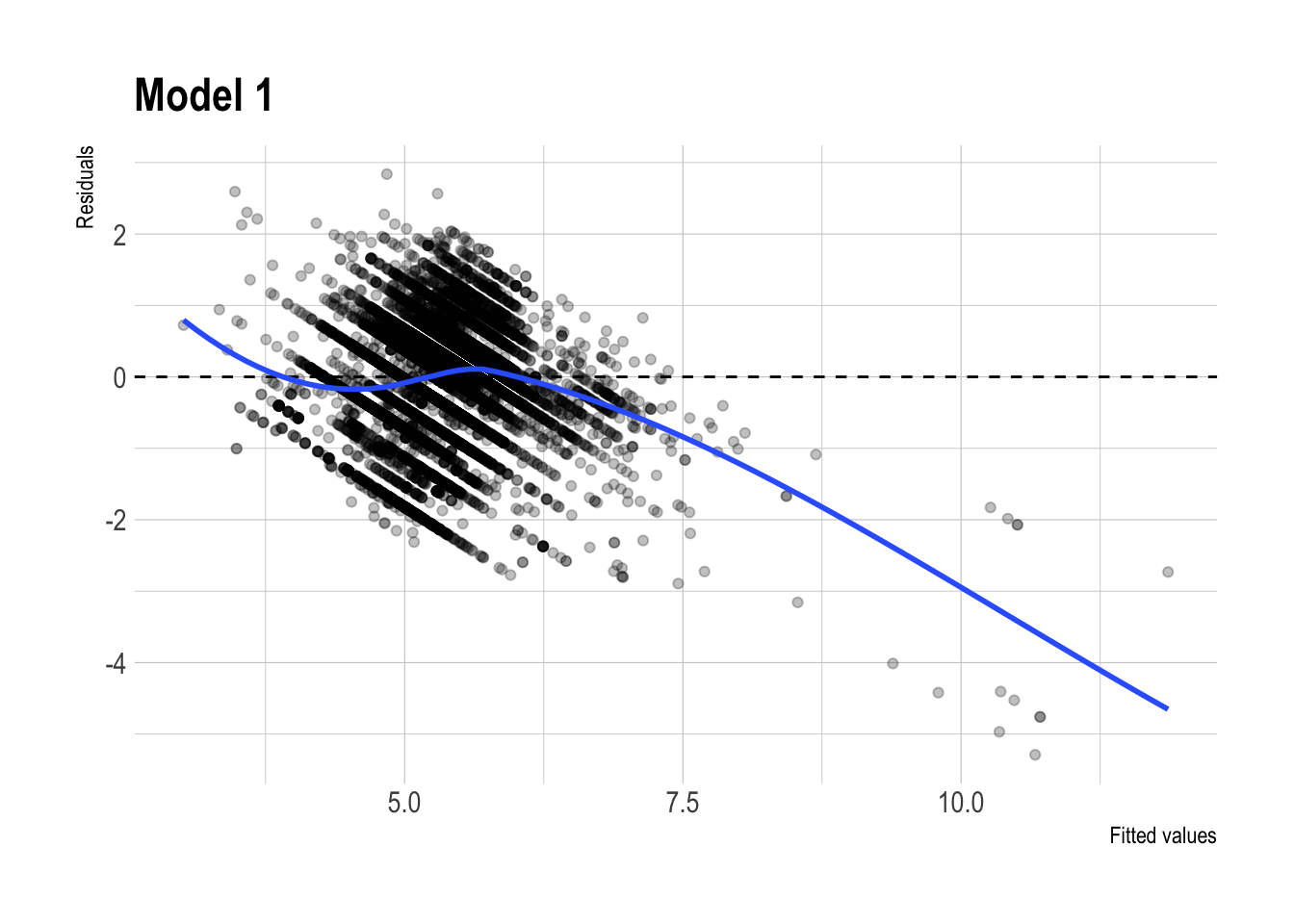
Residual Plots
m1 |>
  augment(newdata = dtest) |>
  ggplot(aes(x = .fitted,
             y = .resid)) +
  geom_point(alpha = 0.25) +
  geom_hline(yintercept = 0, linetype = "dashed") +
  geom_smooth(se = FALSE, method = "loess") +
  labs(
    x = "Fitted values",
    y = "Residuals",
    title = "Model 1"
  )
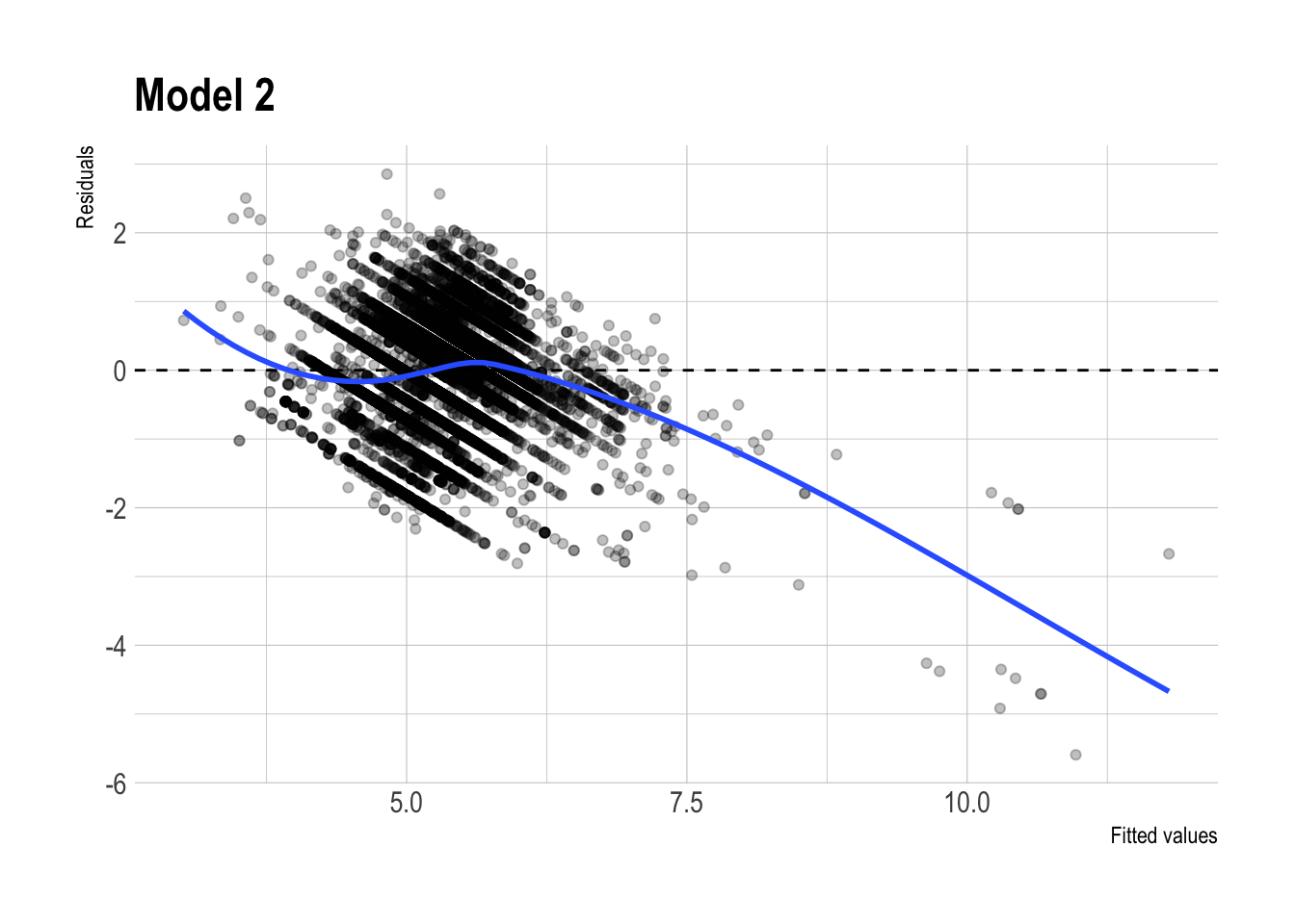
m2 |>
  augment(newdata = dtest) |>
  ggplot(aes(x = .fitted,
             y = .resid)) +
  geom_point(alpha = 0.25) +
  geom_hline(yintercept = 0, linetype = "dashed") +
  geom_smooth(se = FALSE, method = "loess") +
  labs(
    x = "Fitted values",
    y = "Residuals",
    title = "Model 2"
  )
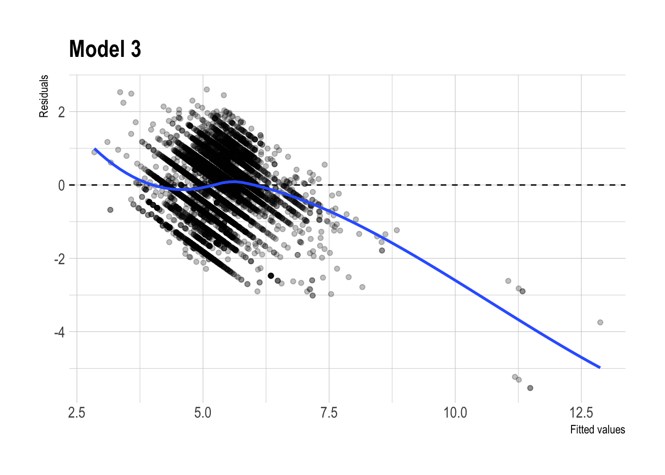
m3 |>
  augment(newdata = dtest) |>
  ggplot(aes(x = .fitted,
             y = .resid)) +
  geom_point(alpha = 0.25) +
  geom_hline(yintercept = 0, linetype = "dashed") +
  geom_smooth(se = FALSE, method = "loess") +
  labs(
    x = "Fitted values",
    y = "Residuals",
    title = "Model 3"
  )
pred_lasso |>
  ggplot(aes(x = .fitted_m1_lasso_1se,
             y = .resid_m1_lasso_1se)) +
  geom_point(alpha = 0.25) +
  geom_hline(yintercept = 0, linetype = "dashed") +
  geom_smooth(se = FALSE, method = "loess") +
  labs(
    x = "Fitted values",
    y = "Residuals",
    title = "Lasso Model 1 (lambda.1se)"
  )
pred_lasso |>
  ggplot(aes(x = .fitted_m1_lasso_min,
             y = .resid_m1_lasso_min)) +
  geom_point(alpha = 0.25) +
  geom_hline(yintercept = 0, linetype = "dashed") +
  geom_smooth(se = FALSE, method = "loess") +
  labs(
    x = "Fitted values",
    y = "Residuals",
    title = "Lasso Model 1 (lambda.min)"
  )
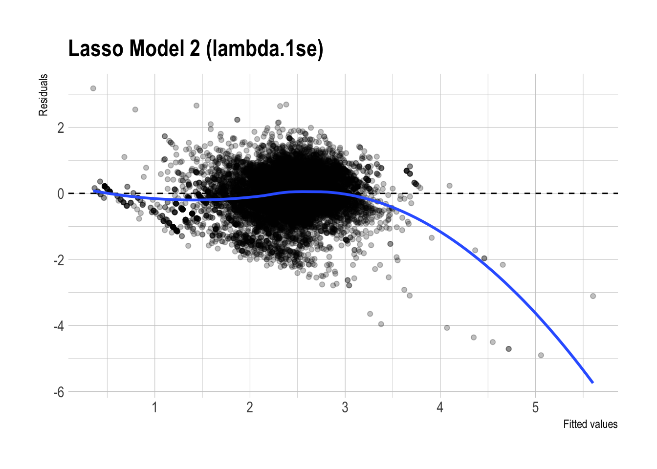
pred_lasso |>
  ggplot(aes(x = .fitted_m2_lasso_1se,
             y = .resid_m2_lasso_1se)) +
  geom_point(alpha = 0.25) +
  geom_hline(yintercept = 0, linetype = "dashed") +
  geom_smooth(se = FALSE, method = "loess") +
  labs(
    x = "Fitted values",
    y = "Residuals",
    title = "Lasso Model 2 (lambda.1se)"
  )
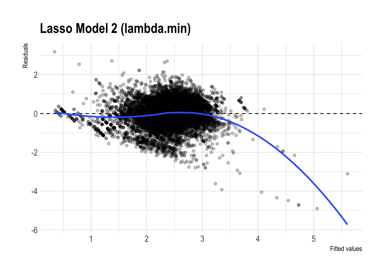
pred_lasso |>
  ggplot(aes(x = .fitted_m2_lasso_min,
             y = .resid_m2_lasso_min)) +
  geom_point(alpha = 0.25) +
  geom_hline(yintercept = 0, linetype = "dashed") +
  geom_smooth(se = FALSE, method = "loess") +
  labs(
    x = "Fitted values",
    y = "Residuals",
    title = "Lasso Model 2 (lambda.min)"
  )
pred_lasso |>
  ggplot(aes(x = .fitted_m3_lasso_1se,
             y = .resid_m3_lasso_1se)) +
  geom_point(alpha = 0.25) +
  geom_hline(yintercept = 0, linetype = "dashed") +
  geom_smooth(se = FALSE, method = "loess") +
  labs(
    x = "Fitted values",
    y = "Residuals",
    title = "Lasso Model 3 (lambda.1se)"
  )
pred_lasso |>
  ggplot(aes(x = .fitted_m3_lasso_min,
             y = .resid_m3_lasso_min)) +
  geom_point(alpha = 0.25) +
  geom_hline(yintercept = 0, linetype = "dashed") +
  geom_smooth(se = FALSE, method = "loess") +
  labs(
    x = "Fitted values",
    y = "Residuals",
    title = "Lasso Model 3 (lambda.min)"
  )
✅ Preferred model: Lasso Model 3 (\(\lambda_{1se}\))
I would prefer Lasso Model 3 (\(\lambda_{1se}\)), but with a more cautious interpretation than claiming it is dramatically better than the unpenalized models.
Out-of-sample performance (test RMSE):
Lasso models have test RMSE around \(0.51\), while the regular linear models have RMSE around \(0.57\).
This indicates that the lasso models perform somewhat better out of sample, but the gap is not huge. So the evidence suggests a modest improvement in predictive performance, not a dramatic one.Interpretability / simplicity + substantively meaningful design:
Model 3 includes substantively meaningful structure, such as brand-specific price sensitivity, promotion effects, and a large demographic design to control for heterogeneity.
Even though Model 3 begins with 3,695 predictors, using \(\lambda_{1se}\) makes the model more conservative by shrinking weak terms to \(0\). This helps produce a model that remains substantively rich, while also being simpler and less cluttered than the fully unpenalized version.
As a supporting diagnostic:
- Residual plot patterns:
- The residual plots for the regular and lasso versions of Model 3 look fairly similar overall. Both show some systematic curvature, especially at higher fitted values, so neither model appears to eliminate all remaining structure in the errors.
- That said, the lasso version looks slightly cleaner, with somewhat less visible patterning. This is consistent with the idea that regularization may improve stability, but the visual difference is not large enough to claim a dramatic improvement.
- The residual plots for the regular and lasso versions of Model 3 look fairly similar overall. Both show some systematic curvature, especially at higher fitted values, so neither model appears to eliminate all remaining structure in the errors.
Bottom line: For estimating elasticities, I would still prefer Lasso Model 3 (\(\lambda_{1se}\)) because it keeps the substantively meaningful interactions and demographic controls while offering slightly better out-of-sample performance and a somewhat simpler specification. However, the lasso and unpenalized models appear more similar than different, so the main advantage of lasso here is modest improvement plus less unnecessary complexity, rather than a major jump in performance.