library(tidyverse)
library(broom)
library(stargazer)
library(rmarkdown)
library(margins)
library(yardstick)
library(WVPlots)
library(pROC)Homework 2
Regression · Quarto Blogging
Directions
Submit your Quarto document for Part 1 to Brightspace using this filename format:
danl-320-hw2-LASTNAME-FIRSTNAME.qmd
(e.g.,danl-320-hw2-choe-byeonghak.qmd)
Due: March 2, 2026, 3:30 PM (ET)
Questions? Email Byeong-Hak bchoe@geneseo.edu.
Required R Packages
Part 1. Regression

Consider the homes DataFrame from the 2004 American Housing Survey, which includes data on home values, demographics, schools, income, finance, mortgages, sales, neighborhood characteristics, noise, smells, state geography, and urban classification.
homes <- read_csv(
  'https://bcdanl.github.io/data/american_housing_survey.csv'
)

homes <- homes |>
  mutate(GT20DWN = ifelse((LPRICE - AMMORT) / LPRICE > 0.2,
                          1, 0)
         )
Variable Description
| Variable | Description |
|---|---|
LPRICE |
Purchase price of unit and land |
VALUE |
Current market value of unit |
STATE |
State code |
METRO |
Central city/suburban status |
ZINC2 |
Household income |
HHGRAD |
Educational level of householder |
BATHS |
Number of full bathrooms in unit |
BEDRMS |
Number of bedrooms in unit |
PER |
Number of persons in household |
ZADULT |
Number of adults (18+) in household |
NUNITS |
Number of units in building |
EAPTBL |
Apartment buildings within 1/2 block of unit |
ECOM1 |
Business/institutions within 1/2 block |
ECOM2 |
Factories/other industry within 1/2 block |
EGREEN |
Open spaces within 1/2 block of unit |
EJUNK |
Trash/junk in streets/properties in 1/2 block |
ELOW1 |
Single-family town/rowhouses in 1/2 block |
ESFD |
Single-family homes within 1/2 block |
ETRANS |
RR/airport/4-lane highway within 1/2 block |
EABAN |
Abandoned/vandalized buildings within 1/2 block |
HOWH |
Rating of unit as a place to live |
HOWN |
Rating of neighborhood as a place to live |
ODORA |
Neighborhood has bad smells |
STRNA |
Neighborhood has heavy street noise/traffic |
FRSTHO |
First home |
AMMORT |
Amount of 1st mortgage when acquired |
INTW |
Interest rate of 1st mortgage (whole number %) |
MATBUY |
Got 1st mortgage in the same year bought unit |
DWNPAY |
Main source of down payment on unit |
Question 1
Plot some relationships and tell a story.
Show answer
# install.packages(c("ggcorrheatmap", "fastDummies"))
library(ggcorrheatmap)
library(fastDummies)

homes_dummy <- homes |>
  select(-STATE) |>
  dummy_cols() |>
  select_if(is.numeric)

ggcorrhm(homes_dummy,
         layout = "bottomright") +
  guides(fill = guide_colorbar(
    theme = theme(
      legend.key.width  = unit(0.5, "lines"),
      legend.key.height = unit(10, "lines")
)))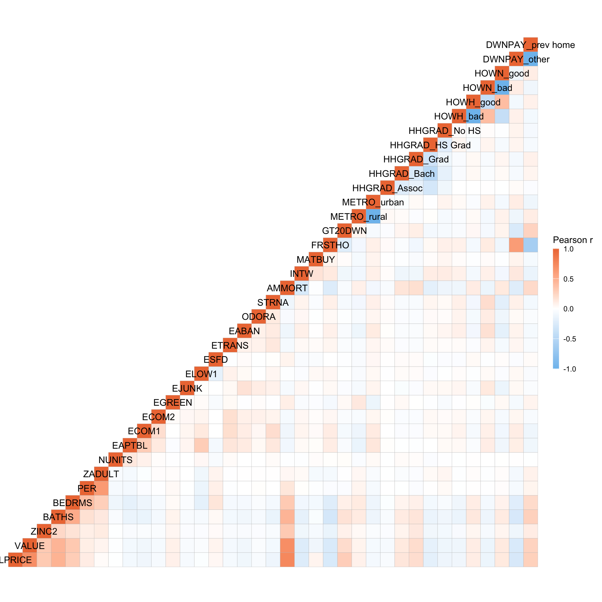
LPRICE/VALUEandAMMORTare positive correlated.FRSTHOandDWNPAY_otherare positively correlated.FRSTHOandDWNPAY_prev_homeare negatively correlated.
Note
- More details on
ggcorrheatmapis: https://leod123.github.io/ggcorrheatmap
Question 2
- Fit a linear regression model with the following specifications:
- Outcome variable: \(\log(VALUE)\)
- Predictors: all but
AMMORTandLPRICE
Show answer
Checking-out Data
glimpse(homes)Rows: 15,565
Columns: 30
$ LPRICE <dbl> 85000, 76500, 93900, 100000, 100000, 96000, 130500, 120000, 19…
$ VALUE <dbl> 150000, 130000, 135000, 140000, 135000, 125000, 135000, 130000…
$ STATE <chr> "GA", "GA", "GA", "GA", "GA", "GA", "GA", "GA", "GA", "GA", "G…
$ METRO <chr> "rural", "rural", "rural", "rural", "rural", "rural", "rural",…
$ ZINC2 <dbl> 15600, 61001, 38700, 80000, 61000, 265000, 42000, 87000, 87800…
$ HHGRAD <chr> "No HS", "HS Grad", "HS Grad", "No HS", "HS Grad", "Bach", "Ba…
$ BATHS <dbl> 2, 2, 2, 3, 2, 2, 2, 2, 3, 2, 2, 1, 2, 2, 2, 2, 2, 2, 2, 1, 3,…
$ BEDRMS <dbl> 3, 3, 3, 4, 3, 3, 3, 4, 3, 3, 3, 3, 4, 3, 3, 3, 3, 3, 3, 4, 5,…
$ PER <dbl> 1, 5, 4, 2, 2, 2, 1, 2, 4, 3, 2, 4, 4, 3, 4, 1, 3, 1, 1, 5, 5,…
$ ZADULT <dbl> 1, 2, 2, 2, 2, 2, 1, 2, 2, 1, 2, 2, 3, 3, 3, 1, 2, 1, 1, 4, 2,…
$ NUNITS <dbl> 1, 1, 1, 1, 1, 1, 1, 1, 1, 1, 1, 1, 1, 1, 1, 1, 1, 1, 1, 1, 1,…
$ EAPTBL <dbl> 0, 0, 0, 0, 0, 0, 0, 0, 0, 0, 0, 0, 0, 0, 0, 0, 0, 0, 0, 0, 0,…
$ ECOM1 <dbl> 0, 0, 0, 0, 1, 0, 0, 0, 0, 0, 0, 0, 0, 0, 0, 0, 0, 0, 0, 1, 0,…
$ ECOM2 <dbl> 0, 0, 0, 0, 0, 0, 0, 0, 0, 0, 0, 0, 0, 0, 0, 0, 0, 0, 0, 0, 0,…
$ EGREEN <dbl> 1, 0, 0, 0, 1, 0, 1, 1, 1, 1, 1, 0, 1, 0, 0, 1, 1, 1, 0, 0, 0,…
$ EJUNK <dbl> 0, 0, 0, 0, 0, 0, 0, 0, 0, 0, 0, 0, 0, 0, 0, 0, 0, 0, 0, 0, 0,…
$ ELOW1 <dbl> 0, 0, 0, 1, 0, 0, 0, 0, 0, 0, 0, 0, 0, 0, 0, 0, 0, 0, 0, 0, 0,…
$ ESFD <dbl> 1, 1, 1, 1, 1, 1, 1, 1, 1, 1, 1, 1, 0, 1, 1, 1, 1, 1, 1, 1, 1,…
$ ETRANS <dbl> 0, 0, 0, 0, 0, 0, 0, 0, 0, 0, 0, 0, 0, 0, 0, 0, 0, 0, 0, 1, 0,…
$ EABAN <dbl> 0, 0, 0, 0, 0, 0, 0, 0, 0, 0, 0, 0, 0, 0, 0, 0, 0, 0, 0, 0, 0,…
$ HOWH <chr> "good", "good", "good", "good", "good", "good", "good", "good"…
$ HOWN <chr> "good", "bad", "good", "good", "good", "good", "good", "good",…
$ ODORA <dbl> 0, 0, 0, 0, 0, 0, 0, 0, 0, 0, 0, 0, 0, 0, 0, 0, 0, 0, 0, 0, 0,…
$ STRNA <dbl> 0, 1, 0, 1, 0, 0, 0, 0, 0, 0, 0, 0, 0, 0, 0, 0, 0, 0, 0, 0, 0,…
$ AMMORT <dbl> 50000, 70000, 117000, 100000, 100000, 96000, 130500, 120000, 1…
$ INTW <dbl> 9, 5, 6, 7, 4, 7, 5, 5, 5, 4, 6, 6, 6, 5, 9, 5, 5, 5, 5, 5, 6,…
$ MATBUY <dbl> 1, 1, 0, 1, 1, 1, 1, 1, 1, 1, 1, 1, 1, 1, 1, 1, 1, 0, 1, 0, 0,…
$ DWNPAY <chr> "other", "other", "other", "prev home", "other", "prev home", …
$ FRSTHO <dbl> 0, 1, 1, 0, 1, 0, 1, 1, 0, 0, 1, 1, 1, 0, 1, 1, 1, 1, 0, 1, 0,…
$ GT20DWN <dbl> 1, 0, 0, 0, 0, 0, 0, 0, 0, 0, 0, 0, 0, 0, 0, 0, 1, 0, 0, 0, 1,…homes |>
count(STATE)# A tibble: 13 × 2
STATE n
<chr> <int>
1 CA 1426
2 CO 1807
3 CT 1422
4 GA 1457
5 IL 237
6 IN 1492
7 LA 779
8 MO 1047
9 OH 1189
10 OK 1173
11 PA 1039
12 TX 1094
13 WA 1403homes |>
count(METRO)# A tibble: 2 × 2
METRO n
<chr> <int>
1 rural 12140
2 urban 3425homes |>
count(BEDRMS) # can be either continuous or categorical.# A tibble: 9 × 2
BEDRMS n
<dbl> <int>
1 0 2
2 1 197
3 2 2210
4 3 7888
5 4 4322
6 5 812
7 6 114
8 7 16
9 8 4homes |>
count(HOWH)# A tibble: 2 × 2
HOWH n
<chr> <int>
1 bad 1275
2 good 14290homes |>
count(HOWN)# A tibble: 2 × 2
HOWN n
<chr> <int>
1 bad 2065
2 good 13500homes |>
count(DWNPAY)# A tibble: 2 × 2
DWNPAY n
<chr> <int>
1 other 10272
2 prev home 5293Training-Test Split
set.seed(1)
homes <- homes |>
  mutate(rnd = runif(n())) |>
  mutate(
    BEDRMS_cat = case_when(
      BEDRMS <= 1 ~ "1 or fewer",
      BEDRMS == 2 ~ "2",
      BEDRMS == 3 ~ "3",
      BEDRMS == 4 ~ "4",
      BEDRMS >= 5 ~ "5+"
    ),
    BEDRMS_cat = factor(BEDRMS_cat)
  )

dtrain <- homes |>
  filter(rnd > .25) |>
  select(-rnd)

dtest <- homes |>
  filter(rnd <= .25) |>
  select(-rnd)
Fitting the Model
m1 <- lm(log(VALUE) ~ .,
        data = dtrain |> select(-AMMORT, -LPRICE, -GT20DWN, -BEDRMS)
        )

stargazer(m1, type = "html")| Dependent variable: | |
| log(VALUE) | |
| STATECO | -0.304*** |
| (0.034) | |
| STATECT | -0.359*** |
| (0.035) | |
| STATEGA | -0.659*** |
| (0.036) | |
| STATEIL | -0.879*** |
| (0.067) | |
| STATEIN | -0.799*** |
| (0.035) | |
| STATELA | -0.746*** |
| (0.042) | |
| STATEMO | -0.691*** |
| (0.039) | |
| STATEOH | -0.698*** |
| (0.038) | |
| STATEOK | -1.030*** |
| (0.037) | |
| STATEPA | -0.896*** |
| (0.039) | |
| STATETX | -1.084*** |
| (0.039) | |
| STATEWA | -0.126*** |
| (0.035) | |
| METROurban | 0.085*** |
| (0.021) | |
| ZINC2 | 0.00000*** |
| (0.00000) | |
| HHGRADBach | 0.129*** |
| (0.026) | |
| HHGRADGrad | 0.213*** |
| (0.030) | |
| HHGRADHS Grad | -0.065*** |
| (0.025) | |
| HHGRADNo HS | -0.165*** |
| (0.037) | |
| BATHS | 0.205*** |
| (0.013) | |
| PER | 0.013* |
| (0.007) | |
| ZADULT | -0.026** |
| (0.012) | |
| NUNITS | -0.001** |
| (0.001) | |
| EAPTBL | -0.035 |
| (0.027) | |
| ECOM1 | -0.015 |
| (0.022) | |
| ECOM2 | -0.094* |
| (0.055) | |
| EGREEN | 0.008 |
| (0.016) | |
| EJUNK | -0.150** |
| (0.058) | |
| ELOW1 | 0.046* |
| (0.027) | |
| ESFD | 0.327*** |
| (0.034) | |
| ETRANS | -0.011 |
| (0.029) | |
| EABAN | -0.180*** |
| (0.041) | |
| HOWHgood | 0.148*** |
| (0.030) | |
| HOWNgood | 0.107*** |
| (0.025) | |
| ODORA | 0.010 |
| (0.038) | |
| STRNA | -0.040** |
| (0.018) | |
| INTW | -0.043*** |
| (0.005) | |
| MATBUY | -0.027* |
| (0.016) | |
| DWNPAYprev home | 0.133*** |
| (0.020) | |
| FRSTHO | -0.091*** |
| (0.020) | |
| BEDRMS_cat2 | 0.199*** |
| (0.072) | |
| BEDRMS_cat3 | 0.297*** |
| (0.071) | |
| BEDRMS_cat4 | 0.388*** |
| (0.073) | |
| BEDRMS_cat5+ | 0.450*** |
| (0.080) | |
| Constant | 11.542*** |
| (0.096) | |
| Observations | 11,690 |
| R2 | 0.311 |
| Adjusted R2 | 0.309 |
| Residual Std. Error | 0.812 (df = 11646) |
| F Statistic | 122.331*** (df = 43; 11646) |
| Note: | p<0.1; p<0.05; p<0.01 |
Question 3
- Refit the linear regression model, retaining only statistically significant predictors from Question 2.
- Compare the revised model to the initial model from Question 2 using:
- \(\beta\) estimates
- \(R^2\)
- RMSE
- Residual plots
Show answer
m1_beta <- m1 |>
  tidy(conf.int = T) |>
  mutate(
    stars = case_when(
      p.value < .01 ~ "***",  # smallest p-values first
      p.value < .05 ~ "**",
      p.value < .1 ~ "*",
      TRUE ~ ""
    ),
    .after = estimate
  )

m1_beta_nostars <- m1_beta |>
  filter(stars == "")

m2 <- lm(log(VALUE) ~ .,
        data = dtrain |> select(-AMMORT, -LPRICE, -GT20DWN, -BEDRMS,
                                -m1_beta_nostars$term)
        )

stargazer(m1, m2, type = "html")| Dependent variable: | ||
| log(VALUE) | ||
| (1) | (2) | |
| STATECO | -0.304*** | -0.303*** |
| (0.034) | (0.034) | |
| STATECT | -0.359*** | -0.358*** |
| (0.035) | (0.035) | |
| STATEGA | -0.659*** | -0.660*** |
| (0.036) | (0.035) | |
| STATEIL | -0.879*** | -0.880*** |
| (0.067) | (0.067) | |
| STATEIN | -0.799*** | -0.798*** |
| (0.035) | (0.035) | |
| STATELA | -0.746*** | -0.748*** |
| (0.042) | (0.042) | |
| STATEMO | -0.691*** | -0.692*** |
| (0.039) | (0.038) | |
| STATEOH | -0.698*** | -0.700*** |
| (0.038) | (0.037) | |
| STATEOK | -1.030*** | -1.027*** |
| (0.037) | (0.037) | |
| STATEPA | -0.896*** | -0.895*** |
| (0.039) | (0.039) | |
| STATETX | -1.084*** | -1.082*** |
| (0.039) | (0.039) | |
| STATEWA | -0.126*** | -0.126*** |
| (0.035) | (0.035) | |
| METROurban | 0.085*** | 0.080*** |
| (0.021) | (0.020) | |
| ZINC2 | 0.00000*** | 0.00000*** |
| (0.00000) | (0.00000) | |
| HHGRADBach | 0.129*** | 0.130*** |
| (0.026) | (0.026) | |
| HHGRADGrad | 0.213*** | 0.214*** |
| (0.030) | (0.030) | |
| HHGRADHS Grad | -0.065*** | -0.065*** |
| (0.025) | (0.025) | |
| HHGRADNo HS | -0.165*** | -0.166*** |
| (0.037) | (0.037) | |
| BATHS | 0.205*** | 0.206*** |
| (0.013) | (0.013) | |
| PER | 0.013* | 0.013* |
| (0.007) | (0.007) | |
| ZADULT | -0.026** | -0.026** |
| (0.012) | (0.012) | |
| NUNITS | -0.001** | -0.001** |
| (0.001) | (0.001) | |
| EAPTBL | -0.035 | |
| (0.027) | ||
| ECOM1 | -0.015 | |
| (0.022) | ||
| ECOM2 | -0.094* | -0.108** |
| (0.055) | (0.053) | |
| EGREEN | 0.008 | |
| (0.016) | ||
| EJUNK | -0.150** | -0.150*** |
| (0.058) | (0.058) | |
| ELOW1 | 0.046* | 0.036 |
| (0.027) | (0.026) | |
| ESFD | 0.327*** | 0.327*** |
| (0.034) | (0.034) | |
| ETRANS | -0.011 | |
| (0.029) | ||
| EABAN | -0.180*** | -0.184*** |
| (0.041) | (0.041) | |
| HOWHgood | 0.148*** | 0.146*** |
| (0.030) | (0.030) | |
| HOWNgood | 0.107*** | 0.110*** |
| (0.025) | (0.025) | |
| ODORA | 0.010 | |
| (0.038) | ||
| STRNA | -0.040** | -0.044** |
| (0.018) | (0.018) | |
| INTW | -0.043*** | -0.043*** |
| (0.005) | (0.005) | |
| MATBUY | -0.027* | -0.027* |
| (0.016) | (0.016) | |
| DWNPAYprev home | 0.133*** | 0.134*** |
| (0.020) | (0.020) | |
| FRSTHO | -0.091*** | -0.093*** |
| (0.020) | (0.020) | |
| BEDRMS_cat2 | 0.199*** | 0.206*** |
| (0.072) | (0.071) | |
| BEDRMS_cat3 | 0.297*** | 0.307*** |
| (0.071) | (0.071) | |
| BEDRMS_cat4 | 0.388*** | 0.398*** |
| (0.073) | (0.073) | |
| BEDRMS_cat5+ | 0.450*** | 0.459*** |
| (0.080) | (0.080) | |
| Constant | 11.542*** | 11.531*** |
| (0.096) | (0.095) | |
| Observations | 11,690 | 11,690 |
| R2 | 0.311 | 0.311 |
| Adjusted R2 | 0.309 | 0.309 |
| Residual Std. Error | 0.812 (df = 11646) | 0.812 (df = 11651) |
| F Statistic | 122.331*** (df = 43; 11646) | 138.363*** (df = 38; 11651) |
| Note: | p<0.1; p<0.05; p<0.01 | |
\(\beta\) estimates
m2_beta <- m2 |>
  tidy(conf.int = T) |>
  mutate(
    stars = case_when(
      p.value < .01 ~ "***",  # smallest p-values first
      p.value < .05 ~ "**",
      p.value < .1 ~ "*",
      TRUE ~ ""
    ),
    .after = estimate
  )

m1_beta <- m1_beta |>
  select(term, estimate, stars, starts_with("conf")) |>
  mutate(model = "long",
         .before = 1)

m2_beta <- m2_beta |>
  select(term, estimate, stars, starts_with("conf")) |>
  mutate(model = "short",
         .before = 1)

betas_linear <- m1_beta |>
  bind_rows(m2_beta) |>
  arrange(term, model)


betas_linear |>
  filter(!str_detect(term, "Intercept")) |>
  ggplot(
    aes(
      y = term,
      x = estimate,
      xmin = conf.low,
      xmax = conf.high,
      color = model
    )
  ) +
    geom_vline(xintercept = 0, color = "maroon", linetype = 2) +
    geom_pointrange(
      position = position_dodge(width = 0.6)
    ) +
    labs(
      title = "Beta Estimates",
      color = "Model",
      y = ""
) 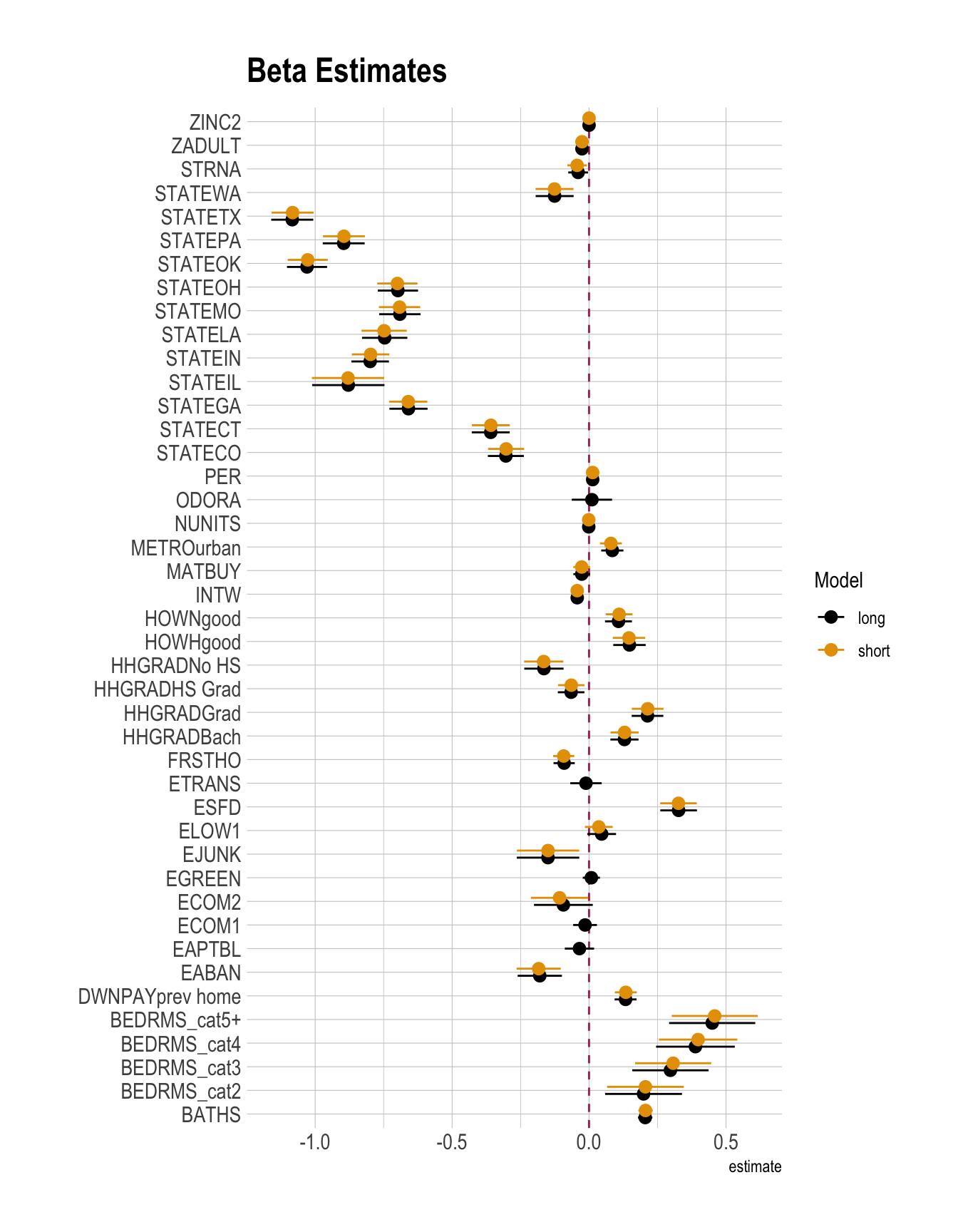
- Beta estimates look almost same.
\(R^2\) / AIC
m1_fit <- m1 |>
  glance()

m2_fit <- m2 |>
  glance()

m1_fit <- m1_fit |>
  mutate(model = "long",
         .before = 1)

m2_fit <- m2_fit |>
  mutate(model = "short",
         .before = 1)

m_fit <- m1_fit |>
  bind_rows(m2_fit)

m_fit |>
paged_table()- In terms of AIC, the short model (
m1) is a slightly better, more parsimonious model that fits the data better with less overfitting.
RMSE
dtest_resid <- dtest |>
  mutate(pred_1 = predict(m1, newdata = dtest),
         pred_2 = predict(m2, newdata = dtest),
         resid_1 = log(VALUE) - pred_1,
         resid_2 = log(VALUE) - pred_2
         ) |>
  select(VALUE,
         pred_1, pred_2,
         resid_1, resid_2)

RMSEs <- dtest_resid |>
  summarise(rmse_1 = sqrt(mean(resid_1^2)),
            rmse_2 = sqrt(mean(resid_2^2)),
            )

RMSEs |>
paged_table()- In terms of RMSE, the long model (
m1) is a slightly better model, as a smaller RMSE reflects smaller differences between predicted and observed values.
Residual plots
dtest_resid |>
  ggplot(aes(x = pred_1, y = resid_1)) +
  geom_point(alpha = 0.25) +
  geom_hline(yintercept = 0, linetype = "dashed") +
  geom_smooth(se = FALSE, method = "loess") +
  labs(
    x = "Fitted values",
    y = "Residuals",
    title = "Residual Plot for Long Model"
  )
dtest_resid |>
  ggplot(aes(x = pred_2, y = resid_2)) +
  geom_point(alpha = 0.25) +
  geom_hline(yintercept = 0, linetype = "dashed") +
  geom_smooth(se = FALSE, method = "loess") +
  labs(
    x = "Fitted values",
    y = "Residuals",
    title = "Residual Plot for Short Model"
  )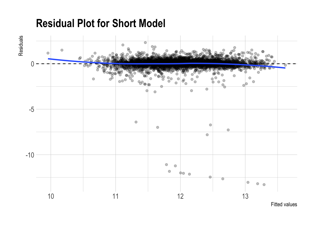
- Both residual plots look almost identical.
Question 4
Fit a logistic regression model with the following specifications:
- Outcome variable: \(\text{GT20DWN}\) (indicating whether the buyer made a down payment of 20% or more)
- Predictors: All available variables except
AMMORTandLPRICE
The outcome variable is defined as: \[ \begin{align} \text{GT20DWN} \,=\,\begin{cases} 1 & \text{if}\; \frac{\text{LPRICE} - \text{AMMORT}}{\text{LPRICE}} > 0.2 \\ 0 & \text{otherwise} \end{cases} \end{align} \]
Analyze and interpret the following relationships:
The association between first-time homeownership (\(\text{FRSTHO}\)) and the probability of making a 20%+ down payment.
The association between number of bedrooms (\(\text{BEDRMS}\)) and the probability of making a 20%+ down payment.
Show answer
m1_logit <- glm(
  GT20DWN ~ .,
  data = dtrain |> select(-AMMORT, -LPRICE, -VALUE, -BEDRMS),
  family = binomial(link = "logit")
)

stargazer(
  m1_logit,
  type = "html",
  digits = 3,
  title = "Logistic regression (logit): GT20DWN"
)| Dependent variable: | |
| GT20DWN | |
| STATECO | -0.178* |
| (0.095) | |
| STATECT | 0.608*** |
| (0.098) | |
| STATEGA | -0.449*** |
| (0.104) | |
| STATEIL | 0.169 |
| (0.191) | |
| STATEIN | -0.072 |
| (0.101) | |
| STATELA | 0.281** |
| (0.120) | |
| STATEMO | 0.179* |
| (0.109) | |
| STATEOH | 0.497*** |
| (0.105) | |
| STATEOK | -0.269** |
| (0.111) | |
| STATEPA | 0.324*** |
| (0.111) | |
| STATETX | -0.100 |
| (0.116) | |
| STATEWA | 0.091 |
| (0.100) | |
| METROurban | -0.017 |
| (0.061) | |
| ZINC2 | 0.00000 |
| (0.00000) | |
| HHGRADBach | 0.166** |
| (0.075) | |
| HHGRADGrad | 0.274*** |
| (0.083) | |
| HHGRADHS Grad | -0.056 |
| (0.073) | |
| HHGRADNo HS | -0.211* |
| (0.115) | |
| BATHS | 0.325*** |
| (0.038) | |
| PER | -0.123*** |
| (0.021) | |
| ZADULT | 0.012 |
| (0.036) | |
| NUNITS | 0.003* |
| (0.002) | |
| EAPTBL | -0.023 |
| (0.082) | |
| ECOM1 | -0.173*** |
| (0.067) | |
| ECOM2 | -0.329* |
| (0.185) | |
| EGREEN | 0.021 |
| (0.046) | |
| EJUNK | -0.015 |
| (0.185) | |
| ELOW1 | 0.045 |
| (0.077) | |
| ESFD | -0.131 |
| (0.097) | |
| ETRANS | -0.099 |
| (0.089) | |
| EABAN | -0.087 |
| (0.133) | |
| HOWHgood | -0.133 |
| (0.092) | |
| HOWNgood | 0.178** |
| (0.077) | |
| ODORA | 0.051 |
| (0.113) | |
| STRNA | -0.116** |
| (0.055) | |
| INTW | -0.094*** |
| (0.016) | |
| MATBUY | 0.297*** |
| (0.045) | |
| DWNPAYprev home | 0.770*** |
| (0.055) | |
| FRSTHO | -0.403*** |
| (0.059) | |
| BEDRMS_cat2 | 0.425* |
| (0.226) | |
| BEDRMS_cat3 | 0.229 |
| (0.225) | |
| BEDRMS_cat4 | 0.371 |
| (0.230) | |
| BEDRMS_cat5+ | 0.254 |
| (0.248) | |
| Constant | -1.240*** |
| (0.295) | |
| Observations | 11,690 |
| Log Likelihood | -6,417.980 |
| Akaike Inf. Crit. | 12,923.960 |
| Note: | p<0.1; p<0.05; p<0.01 |
m1_logit_betas <- m1_logit |>
  tidy(conf.int = T) |>
  mutate(
    stars = case_when(
      p.value < .01 ~ "***",  # smallest p-values first
      p.value < .05 ~ "**",
      p.value < .1 ~ "*",
      TRUE ~ ""
    ),
    .after = estimate
  )

m1_logit_betas |>
  paged_table()
AME
sum_me <- summary(
  margins(m1_logit,
          variables = c("FRSTHO",
                        "BEDRMS_cat"))
)

sum_me
factor AME SE z p lower upper
BEDRMS_cat2 0.0762 0.0377 2.0221 0.0432 0.0023 0.1501
BEDRMS_cat3 0.0397 0.0373 1.0652 0.2868 -0.0334 0.1128
BEDRMS_cat4 0.0658 0.0384 1.7147 0.0864 -0.0094 0.1411
BEDRMS_cat5+ 0.0442 0.0417 1.0610 0.2887 -0.0375 0.1259
FRSTHO -0.0742 0.0109 -6.8261 0.0000 -0.0955 -0.0529- The relationship between number of bedrooms (\(\text{BEDRMS}\)) and the probability of making a 20%+ down payment:
- On average, homes with two bedrooms are estimated to have a 7.62 percentage point higher probability of a 20% or higher down payment than homes with one bedroom or no bedroom, holding other covariates constant.
- Intuition: Relative to very small homes, two-bedroom homes may be more commonly purchased by households with greater financial resources, making a larger down payment more attainable.
- On average, homes with four bedrooms are estimated to have a 6.58 percentage point higher probability of a 20% or higher down payment than homes with one bedroom or no bedroom, holding other covariates constant.
- Intuition: Four-bedroom homes may more often be bought by larger or more financially established households with enough savings to put more money down upfront.
- By contrast, the estimated relationships for homes with three bedrooms and five or more bedrooms are not statistically significant.
- Intuition: Their estimated effects are too imprecise to rule out the possibility that the true differences from the reference group are small or zero.
- On average, homes with two bedrooms are estimated to have a 7.62 percentage point higher probability of a 20% or higher down payment than homes with one bedroom or no bedroom, holding other covariates constant.
- The association between first-time homeownership (\(\text{FRSTHO}\)) and the probability of making a 20%+ down payment:
- On average, first homes have an estimated 7.61 percentage point lower probability of making a 20% or higher down payment than non-first homes, holding other covariates constant.
- Intuition: First-time buyers often have less accumulated savings and fewer housing-related assets (for example, they cannot use equity from selling a previous home), so they are less likely to be able to put down 20% or more.
Question 5
- Refit the logistic regression model, adding interaction terms:
- Predictors: all previously included predictors in Question 4 plus the interaction between \(\text{FRSTHO}\) and \(\text{BEDRMS}\)
- Interpret how the relationship between \(\text{BEDRMS}\) and the probability of a 20%+ down payment varies depending on whether the buyer is a first-time homeowner (\(\text{FRSTHO}\)).
Show answer
m2_logit <- glm(
  GT20DWN ~ . + BEDRMS_cat:FRSTHO,
  data = dtrain |>
    select(-AMMORT, -LPRICE, -VALUE, -BEDRMS),
  family = binomial(link = "logit")
)

stargazer(
  m2_logit,
  type = "html",
  digits = 3,
  title = "Logistic regression (logit): GT20DWN with an Interaction"
)| Dependent variable: | |
| GT20DWN | |
| STATECO | -0.178* |
| (0.095) | |
| STATECT | 0.613*** |
| (0.098) | |
| STATEGA | -0.453*** |
| (0.104) | |
| STATEIL | 0.174 |
| (0.191) | |
| STATEIN | -0.073 |
| (0.101) | |
| STATELA | 0.280** |
| (0.120) | |
| STATEMO | 0.180* |
| (0.109) | |
| STATEOH | 0.498*** |
| (0.105) | |
| STATEOK | -0.267** |
| (0.111) | |
| STATEPA | 0.324*** |
| (0.111) | |
| STATETX | -0.104 |
| (0.116) | |
| STATEWA | 0.095 |
| (0.100) | |
| METROurban | -0.013 |
| (0.061) | |
| ZINC2 | 0.00000 |
| (0.00000) | |
| HHGRADBach | 0.165** |
| (0.075) | |
| HHGRADGrad | 0.272*** |
| (0.083) | |
| HHGRADHS Grad | -0.056 |
| (0.073) | |
| HHGRADNo HS | -0.213* |
| (0.115) | |
| BATHS | 0.323*** |
| (0.038) | |
| PER | -0.125*** |
| (0.021) | |
| ZADULT | 0.017 |
| (0.036) | |
| NUNITS | 0.003 |
| (0.002) | |
| EAPTBL | -0.020 |
| (0.082) | |
| ECOM1 | -0.172** |
| (0.067) | |
| ECOM2 | -0.333* |
| (0.185) | |
| EGREEN | 0.020 |
| (0.046) | |
| EJUNK | -0.013 |
| (0.185) | |
| ELOW1 | 0.044 |
| (0.077) | |
| ESFD | -0.135 |
| (0.097) | |
| ETRANS | -0.099 |
| (0.089) | |
| EABAN | -0.089 |
| (0.133) | |
| HOWHgood | -0.135 |
| (0.092) | |
| HOWNgood | 0.179** |
| (0.077) | |
| ODORA | 0.053 |
| (0.113) | |
| STRNA | -0.114** |
| (0.055) | |
| INTW | -0.094*** |
| (0.016) | |
| MATBUY | 0.297*** |
| (0.045) | |
| DWNPAYprev home | 0.769*** |
| (0.056) | |
| FRSTHO | -0.246 |
| (0.427) | |
| BEDRMS_cat2 | 0.538* |
| (0.320) | |
| BEDRMS_cat3 | 0.291 |
| (0.316) | |
| BEDRMS_cat4 | 0.461 |
| (0.319) | |
| BEDRMS_cat5+ | 0.421 |
| (0.333) | |
| FRSTHO:BEDRMS_cat2 | -0.224 |
| (0.441) | |
| FRSTHO:BEDRMS_cat3 | -0.097 |
| (0.430) | |
| FRSTHO:BEDRMS_cat4 | -0.174 |
| (0.437) | |
| FRSTHO:BEDRMS_cat5+ | -0.713 |
| (0.499) | |
| Constant | -1.317*** |
| (0.366) | |
| Observations | 11,690 |
| Log Likelihood | -6,414.807 |
| Akaike Inf. Crit. | 12,925.610 |
| Note: | p<0.1; p<0.05; p<0.01 |
m2_logit_betas <- m2_logit |>
  tidy(conf.int = T)  |>
  mutate(
    stars = case_when(
      p.value < .01 ~ "***",  # smallest p-values first
      p.value < .05 ~ "**",
      p.value < .1 ~ "*",
      TRUE ~ ""
    ),
    .after = estimate
  )

m2_logit_betas |>
  paged_table()
AME
sum_me2 <- summary(
  margins(m2_logit,
          variables = c("FRSTHO", "BEDRMS_cat"),
          at = list(
            BEDRMS_cat = levels(dtrain$BEDRMS_cat)
            )
    )
)

sum_me2 |>
  paged_table()
at = option in margins()
In this
margins()code, theat =option tells R to compute marginal effects at specific representative values of a predictor rather than averaging over the observed distribution of that predictor.Here,
at = list(BEDRMS_cat = levels(dtrain$BEDRMS_cat))asksmargins()to evaluate the marginal effects at each bedroom category: for example, 1 or fewer, 2, 3, 4, and 5+ bedrooms.This is similar in spirit to the idea of a marginal effect at a representative value (MER) that we discussed in class. The difference is that, instead of evaluating the effect at the mean of a numeric variable, we are evaluating it at each representative category of a factor variable.
This is especially useful when the model includes an interaction, because the marginal effect of one variable may differ depending on the value or category of another variable.
In this example, the
at =option lets us see how the estimated effect ofFRSTHOchanges across bedroom categories, rather than reporting only one overall average marginal effect.So, you can think of
at =as asking: “What is the marginal effect when we fix a predictor at a particular representative value or category?”In our case, it answers: “What is the marginal effect of first-time homebuyer status for homes with 1 or fewer bedrooms, 2 bedrooms, 3 bedrooms, 4 bedrooms, and 5+ bedrooms?”
- The relationship between number of bedrooms (\(\text{BEDRMS}\)) and the probability of making a down payment greater than 20%:
- Relative to homes with one bedroom or no bedroom (the reference group), homes with two bedrooms have an estimated 8.33 percentage point higher probability of making a down payment greater than 20%, on average, holding other covariates constant.
- This estimate is statistically significant at the 5% level (\(p = 0.038\)).
- Intuition: Compared with very small homes, two-bedroom homes may be more likely to be purchased by households with somewhat greater financial stability or savings, making a larger down payment more feasible.
- Relative to homes with one bedroom or no bedroom, homes with three bedrooms have an estimated 4.50 percentage point higher probability of making a down payment greater than 20%, on average, holding other covariates constant.
- However, this estimate is not statistically significant (\(p = 0.256\)).
- Intuition: Although the estimated association is positive, the evidence is not strong enough to conclude that three-bedroom homes differ meaningfully from the reference group after accounting for the other predictors in the model.
- Relative to homes with one bedroom or no bedroom, homes with four bedrooms have an estimated 7.19 percentage point higher probability of making a down payment greater than 20%, on average, holding other covariates constant.
- This estimate is marginally significant at the 10% level (\(p = 0.077\)), but not at the 5% level.
- Intuition: Four-bedroom homes may be more likely to be purchased by larger or more established households with greater accumulated savings, but the evidence here is only moderately strong.
- Relative to homes with one bedroom or no bedroom, homes with five or more bedrooms have an estimated 3.65 percentage point higher probability of making a down payment greater than 20%, on average, holding other covariates constant.
- This estimate is not statistically significant (\(p = 0.402\)).
- Intuition: While the point estimate is positive, it is too imprecise to conclude that homes with five or more bedrooms are meaningfully different from the reference group.
- Relative to homes with one bedroom or no bedroom (the reference group), homes with two bedrooms have an estimated 8.33 percentage point higher probability of making a down payment greater than 20%, on average, holding other covariates constant.
- The relationship between first-time homebuyer status (\(\text{FRSTHO}\)) and the probability of making a down payment greater than 20%, by bedroom category:
- Among homes with one bedroom or no bedroom, first homes have an estimated 4.05 percentage point lower probability of making a down payment greater than 20% than non-first homes, on average, holding other covariates constant.
- This estimate is not statistically significant (\(p = 0.567\)).
- Intuition: For very small homes, the data do not provide strong evidence that first-time buyers differ from non-first-time buyers in down payment behavior.
- Among homes with two bedrooms, first homes have an estimated 9.00 percentage point lower probability of making a down payment greater than 20% than non-first homes, on average, holding other covariates constant.
- This estimate is statistically significant at the 1% level (\(p < 0.001\)).
- Intuition: First-time buyers of two-bedroom homes may have less accumulated wealth or home equity to put toward a large down payment than repeat buyers.
- Among homes with three bedrooms, first homes have an estimated 6.22 percentage point lower probability of making a down payment greater than 20% than non-first homes, on average, holding other covariates constant.
- This estimate is statistically significant at the 1% level (\(p < 0.001\)).
- Intuition: This pattern is consistent with the idea that repeat buyers can often use proceeds or equity from a previous home sale to make a larger down payment.
- Among homes with four bedrooms, first homes have an estimated 7.94 percentage point lower probability of making a down payment greater than 20% than non-first homes, on average, holding other covariates constant.
- This estimate is statistically significant at the 1% level (\(p < 0.001\)).
- Intuition: For larger homes, first-time buyers may face greater financing constraints because these homes generally require more upfront cash.
- Among homes with five or more bedrooms, first homes have an estimated 16.13 percentage point lower probability of making a down payment greater than 20% than non-first homes, on average, holding other covariates constant.
- This estimate is statistically significant at the 1% level (\(p < 0.001\)).
- Intuition: The gap is especially large for the biggest homes, suggesting that repeat buyers may have a particularly strong financial advantage in making large down payments in this segment of the housing market.
- Among homes with one bedroom or no bedroom, first homes have an estimated 4.05 percentage point lower probability of making a down payment greater than 20% than non-first homes, on average, holding other covariates constant.
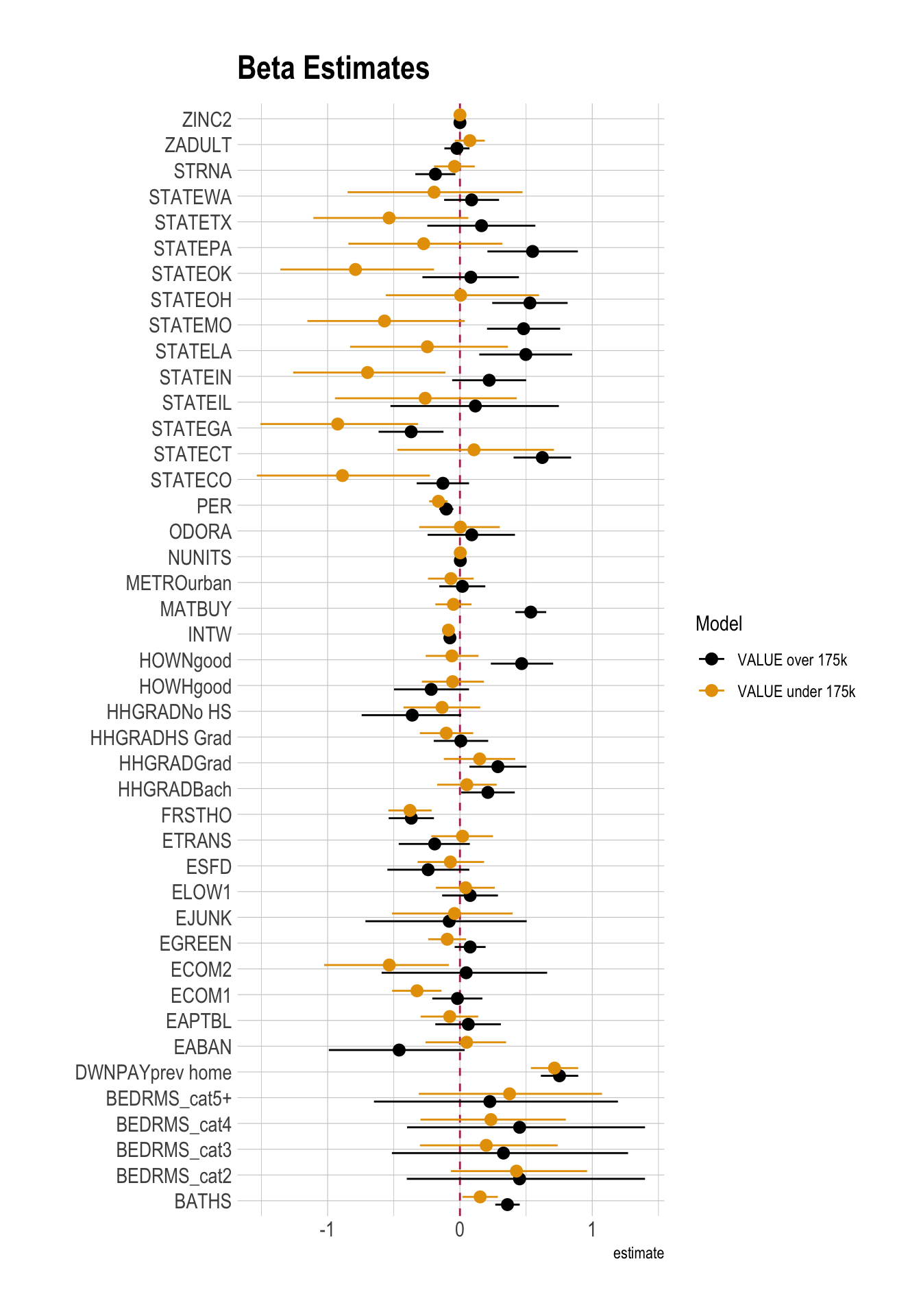
Question 6
- Fit separate logistic regression models (with the same model specification as in Question 4) for two subsets of home data:
- Homes worth \(\text{VALUE} \geq 175k\).
- Homes worth \(\text{VALUE} < 175k\).
- Compare residual deviance, \(RMSE\), and classification performance between the two models.
Show answer
Subsetting Data
dtrain_over_175k <- dtrain |>
  filter(VALUE >= 175000)
dtrain_under_175k <- dtrain |>
  filter(VALUE < 175000)

dtest_over_175k <- dtest |>
  filter(VALUE >= 175000)
dtest_under_175k <- dtest |>
  filter(VALUE < 175000)
Fitting the Models
m1_logit_over_175k <- glm(
  GT20DWN ~ .,
  data = dtrain_over_175k |> select(-AMMORT, -LPRICE, -VALUE, -BEDRMS),
  family = binomial(link = "logit")
)

stargazer(
  m1_logit_over_175k,
  type = "html",
  digits = 3,
  title = "Logistic regression (logit): GT20DWN (VALUE over 175k)"
)| Dependent variable: | |
| GT20DWN | |
| STATECO | -0.129 |
| (0.101) | |
| STATECT | 0.623*** |
| (0.111) | |
| STATEGA | -0.369*** |
| (0.125) | |
| STATEIL | 0.116 |
| (0.323) | |
| STATEIN | 0.221 |
| (0.143) | |
| STATELA | 0.498*** |
| (0.179) | |
| STATEMO | 0.481*** |
| (0.141) | |
| STATEOH | 0.529*** |
| (0.145) | |
| STATEOK | 0.082 |
| (0.186) | |
| STATEPA | 0.549*** |
| (0.174) | |
| STATETX | 0.163 |
| (0.208) | |
| STATEWA | 0.088 |
| (0.106) | |
| METROurban | 0.018 |
| (0.089) | |
| ZINC2 | 0.00000 |
| (0.00000) | |
| HHGRADBach | 0.211** |
| (0.103) | |
| HHGRADGrad | 0.287*** |
| (0.110) | |
| HHGRADHS Grad | 0.007 |
| (0.105) | |
| HHGRADNo HS | -0.361* |
| (0.192) | |
| BATHS | 0.359*** |
| (0.047) | |
| PER | -0.103*** |
| (0.027) | |
| ZADULT | -0.023 |
| (0.048) | |
| NUNITS | 0.003 |
| (0.006) | |
| EAPTBL | 0.063 |
| (0.126) | |
| ECOM1 | -0.019 |
| (0.096) | |
| ECOM2 | 0.047 |
| (0.318) | |
| EGREEN | 0.077 |
| (0.060) | |
| EJUNK | -0.081 |
| (0.309) | |
| ELOW1 | 0.077 |
| (0.108) | |
| ESFD | -0.241 |
| (0.158) | |
| ETRANS | -0.191 |
| (0.137) | |
| EABAN | -0.460* |
| (0.261) | |
| HOWHgood | -0.217 |
| (0.145) | |
| HOWNgood | 0.466*** |
| (0.120) | |
| ODORA | 0.089 |
| (0.168) | |
| STRNA | -0.185** |
| (0.077) | |
| INTW | -0.076*** |
| (0.025) | |
| MATBUY | 0.535*** |
| (0.060) | |
| DWNPAYprev home | 0.752*** |
| (0.072) | |
| FRSTHO | -0.367*** |
| (0.087) | |
| BEDRMS_cat2 | 0.450 |
| (0.454) | |
| BEDRMS_cat3 | 0.329 |
| (0.450) | |
| BEDRMS_cat4 | 0.451 |
| (0.454) | |
| BEDRMS_cat5+ | 0.226 |
| (0.466) | |
| Constant | -1.736*** |
| (0.535) | |
| Observations | 5,903 |
| Log Likelihood | -3,508.690 |
| Akaike Inf. Crit. | 7,105.381 |
| Note: | p<0.1; p<0.05; p<0.01 |
m1_logit_betas_over_175k <- m1_logit_over_175k |>
  tidy(conf.int = T) |>
  mutate(
    stars = case_when(
      p.value < .01 ~ "***",  # smallest p-values first
      p.value < .05 ~ "**",
      p.value < .1 ~ "*",
      TRUE ~ ""
    ),
    .after = estimate
  )
m1_logit_under_175k <- glm(
GT20DWN ~ .,
data = dtrain_under_175k |> select(-AMMORT, -LPRICE, -VALUE, -BEDRMS),
family = binomial(link = "logit")
)
stargazer(
m1_logit_under_175k,
type = "html",
digits = 3,
title = "Logistic regression (logit): GT20DWN (VALUE under 175k)"
)| Dependent variable: | |
| GT20DWN | |
| STATECO | -0.888*** |
| (0.333) | |
| STATECT | 0.106 |
| (0.301) | |
| STATEGA | -0.924*** |
| (0.303) | |
| STATEIL | -0.263 |
| (0.349) | |
| STATEIN | -0.698** |
| (0.292) | |
| STATELA | -0.246 |
| (0.303) | |
| STATEMO | -0.570* |
| (0.302) | |
| STATEOH | 0.005 |
| (0.294) | |
| STATEOK | -0.790*** |
| (0.295) | |
| STATEPA | -0.274 |
| (0.296) | |
| STATETX | -0.535* |
| (0.298) | |
| STATEWA | -0.196 |
| (0.336) | |
| METROurban | -0.068 |
| (0.088) | |
| ZINC2 | 0.00000 |
| (0.00000) | |
| HHGRADBach | 0.052 |
| (0.115) | |
| HHGRADGrad | 0.149 |
| (0.138) | |
| HHGRADHS Grad | -0.103 |
| (0.103) | |
| HHGRADNo HS | -0.135 |
| (0.148) | |
| BATHS | 0.153** |
| (0.068) | |
| PER | -0.163*** |
| (0.035) | |
| ZADULT | 0.075 |
| (0.058) | |
| NUNITS | 0.003 |
| (0.002) | |
| EAPTBL | -0.077 |
| (0.111) | |
| ECOM1 | -0.324*** |
| (0.095) | |
| ECOM2 | -0.534** |
| (0.239) | |
| EGREEN | -0.096 |
| (0.073) | |
| EJUNK | -0.042 |
| (0.232) | |
| ELOW1 | 0.043 |
| (0.114) | |
| ESFD | -0.072 |
| (0.128) | |
| ETRANS | 0.020 |
| (0.119) | |
| EABAN | 0.050 |
| (0.155) | |
| HOWHgood | -0.056 |
| (0.120) | |
| HOWNgood | -0.061 |
| (0.102) | |
| ODORA | 0.003 |
| (0.155) | |
| STRNA | -0.041 |
| (0.079) | |
| INTW | -0.087*** |
| (0.021) | |
| MATBUY | -0.049 |
| (0.070) | |
| DWNPAYprev home | 0.714*** |
| (0.091) | |
| FRSTHO | -0.378*** |
| (0.083) | |
| BEDRMS_cat2 | 0.427 |
| (0.261) | |
| BEDRMS_cat3 | 0.199 |
| (0.264) | |
| BEDRMS_cat4 | 0.234 |
| (0.279) | |
| BEDRMS_cat5+ | 0.375 |
| (0.352) | |
| Constant | -0.124 |
| (0.440) | |
| Observations | 5,787 |
| Log Likelihood | -2,836.965 |
| Akaike Inf. Crit. | 5,761.931 |
| Note: | p<0.1; p<0.05; p<0.01 |
m1_logit_betas_under_175k <- m1_logit_under_175k |>
  tidy(conf.int = T) |>
  mutate(
    stars = case_when(
      p.value < .01 ~ "***",  # smallest p-values first
      p.value < .05 ~ "**",
      p.value < .1 ~ "*",
      TRUE ~ ""
    ),
    .after = estimate
  )
Betas
m1_logit_betas_over_175k <- m1_logit_betas_over_175k |>
  select(term, estimate, stars, starts_with("conf")) |>
  mutate(model = "VALUE over 175k",
         .before = 1)

m1_logit_betas_under_175k <- m1_logit_betas_under_175k |>
  select(term, estimate, stars, starts_with("conf")) |>
  mutate(model = "VALUE under 175k",
         .before = 1)

betas_logit_175k <- m1_logit_betas_over_175k |>
  bind_rows(m1_logit_betas_under_175k) |>
  arrange(term, model)


betas_logit_175k |>
  filter(!str_detect(term, "Intercept")) |>
  ggplot(
    aes(
      y = term,
      x = estimate,
      xmin = conf.low,
      xmax = conf.high,
      color = model
    )
  ) +
    geom_vline(xintercept = 0, color = "maroon", linetype = 2) +
    geom_pointrange(
      position = position_dodge(width = 0.6)
    ) +
    labs(
      title = "Beta Estimates",
      color = "Model",
      y = ""
) 
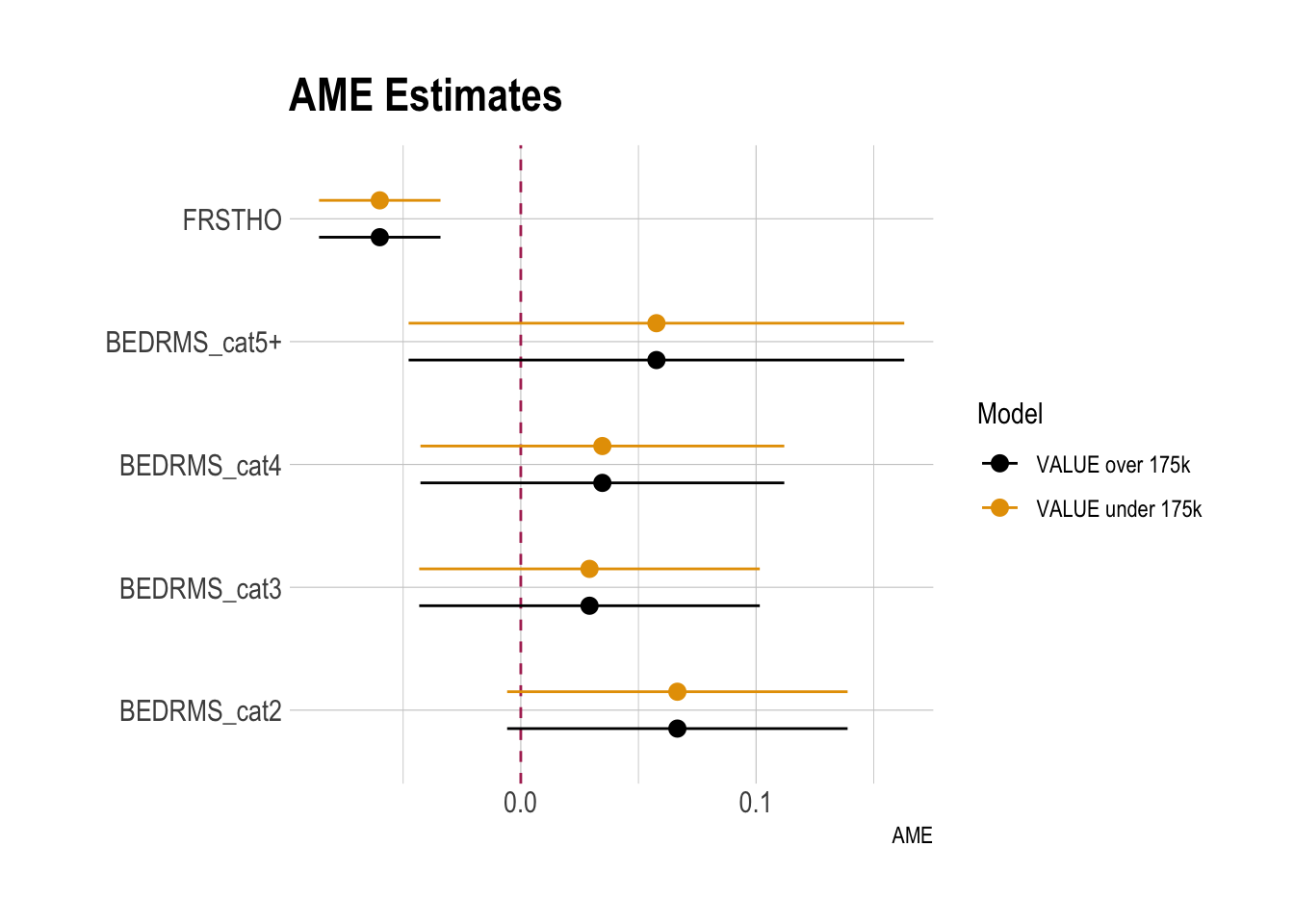
AMEs of FRSTHO and BEDRMS_cat
sum_me_over_175k <- summary(
  margins(m1_logit_under_175k,
          variables = c("FRSTHO", "BEDRMS_cat")
    )
) |>
  mutate(model = "VALUE over 175k",
         .before = 1)

sum_me_under_175k <- summary(
  margins(m1_logit_under_175k,
          variables = c("FRSTHO", "BEDRMS_cat")
    )
) |>
  mutate(model = "VALUE under 175k",
         .before = 1)


AME_logit_175k <- sum_me_over_175k |>
  bind_rows(sum_me_under_175k) |>
  arrange(factor, model)

AME_logit_175k |>
  ggplot(
    aes(
      y = factor,
      x = AME,
      xmin = lower,
      xmax = upper,
      color = model
    )
  ) +
    geom_vline(xintercept = 0, color = "maroon", linetype = 2) +
    geom_pointrange(
      position = position_dodge(width = 0.6)
    ) +
    labs(
      title = "AME Estimates",
      color = "Model",
      y = ""
) 
Residual Deviance
m1_logit_over_175k |>
  glance()  # focus on the `deviance` column
# A tibble: 1 × 8
null.deviance df.null logLik AIC BIC deviance df.residual nobs
<dbl> <int> <dbl> <dbl> <dbl> <dbl> <int> <int>
1 7776. 5902 -3509. 7105. 7399. 7017. 5859 5903m1_logit_under_175k |>
glance() # focus on the `deviance` column# A tibble: 1 × 8
null.deviance df.null logLik AIC BIC deviance df.residual nobs
<dbl> <int> <dbl> <dbl> <dbl> <dbl> <int> <int>
1 6090. 5786 -2837. 5762. 6055. 5674. 5743 5787RMSE
dtest_resid_over_175k <- dtest_over_175k |>
  mutate(.fitted = predict(m1_logit_over_175k,
                           newdata = dtest_over_175k,
                           type = "response"),
         .resid = GT20DWN - .fitted
         ) |>
  select(GT20DWN,
         .fitted, .resid)

dtest_resid_under_175k <- dtest_under_175k |>
  mutate(.fitted = predict(m1_logit_under_175k,
                           newdata = dtest_under_175k,
                           type = "response"),
         .resid = GT20DWN - .fitted
  ) |>
  select(GT20DWN,
         .fitted, .resid)

RMSE_over_175k <- dtest_resid_over_175k |>
  summarise(rmse = sqrt(mean(.resid^2))
            )

RMSE_under_175k <- dtest_resid_under_175k |>
  summarise(rmse = sqrt(mean(.resid^2))
            )

RMSE_over_175k |>
  paged_table()
RMSE_under_175k |>
paged_table()Classification Performance with the Same Threshold
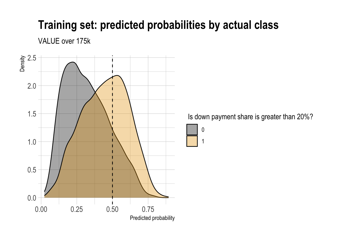
Double Density Plot
threshold_over_175k <- .5

m1_logit_over_175k |>
  augment(type.predict = "response") |>
  ggplot(aes(x = .fitted,
             fill = factor(GT20DWN))) +
  geom_density(alpha = 0.35) +
  geom_vline(xintercept = threshold_over_175k, linetype = "dashed") +
  labs(
    x = "Predicted probability",
    y = "Density",
    fill = " Is down payment share is greater than 20%?",
    title = "Training set: predicted probabilities by actual class",
    subtitle = "VALUE over 175k"
  )
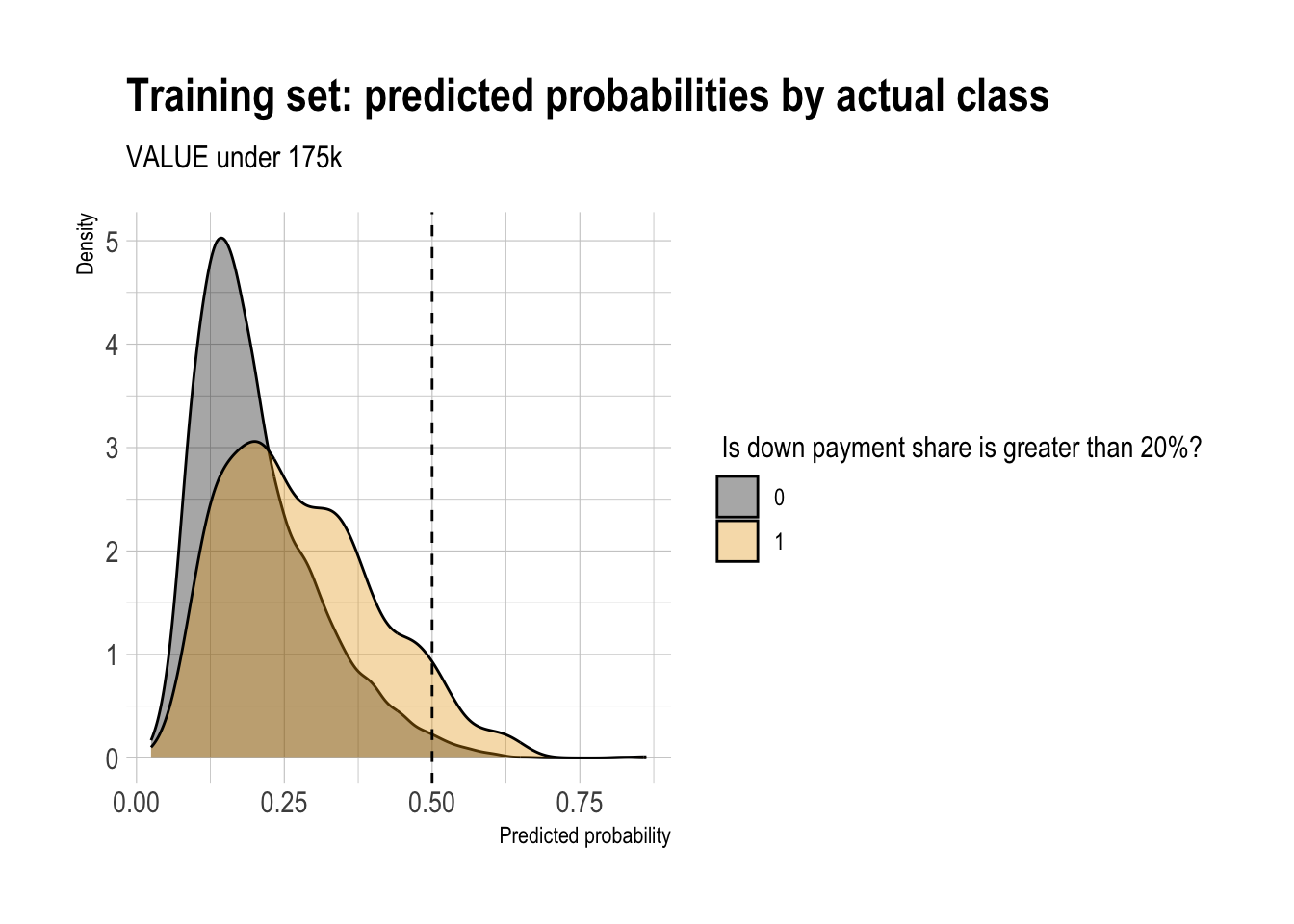
threshold_under_175k <- .5

m1_logit_under_175k |>
  augment(type.predict = "response") |>
  ggplot(aes(x = .fitted,
             fill = factor(GT20DWN))) +
  geom_density(alpha = 0.35) +
  geom_vline(xintercept = threshold_under_175k, linetype = "dashed") +
  labs(
    x = "Predicted probability",
    y = "Density",
    fill = " Is down payment share is greater than 20%?",
    title = "Training set: predicted probabilities by actual class",
    subtitle = "VALUE under 175k"
  )
Confusion Matrix
df_cm_over_175k <- m1_logit_over_175k |>
  augment(newdata = dtest_over_175k,
          type.predict = "response") |>
  mutate(
    actual = factor(GT20DWN,
                    levels = c(0, 1),
                    labels = c("DWN <= 20%", "DWN > 20%")),
    pred   = factor(if_else(.fitted > threshold_over_175k, 1, 0),
                    levels = c(0, 1),
                    labels = c("DWN <= 20%", "DWN > 20%")),
  )

conf_mat_over_175k <- table(truth = df_cm_over_175k$actual,
                            prediction = df_cm_over_175k$pred)
conf_mat_over_175k
prediction
truth DWN <= 20% DWN > 20%
DWN <= 20% 1029 185
DWN > 20% 409 305df_cm_under_175k <- m1_logit_under_175k |>
augment(newdata = dtest_under_175k,
type.predict = "response") |>
mutate(
actual = factor(GT20DWN,
levels = c(0, 1),
labels = c("DWN <= 20%", "DWN > 20%")),
pred = factor(if_else(.fitted > threshold_under_175k, 1, 0),
levels = c(0, 1),
labels = c("DWN <= 20%", "DWN > 20%")),
)
conf_mat_under_175k <- table(truth = df_cm_under_175k$actual,
prediction = df_cm_under_175k$pred)
conf_mat_under_175k prediction
truth DWN <= 20% DWN > 20%
DWN <= 20% 1507 19
DWN > 20% 404 17Performance Metrics
base_rate_over_175k   <- mean(dtest_over_175k$GT20DWN)

accuracy_over_175k <- (conf_mat_over_175k[1,1] + conf_mat_over_175k[2,2]) / sum(conf_mat_over_175k)
precision_over_175k <- conf_mat_over_175k[2,2] / sum(conf_mat_over_175k[,2])
recall_over_175k <- conf_mat_over_175k[2,2] / sum(conf_mat_over_175k[2,])
specificity_over_175k <- conf_mat_over_175k[1,1] / sum(conf_mat_over_175k[1,])
enrichment_over_175k <- precision_over_175k / base_rate_over_175k


df_class_metric_over_175k <-
  data.frame(
    metric = c("Base rate",
               "Accuracy",
               "Precision",
               "Recall",
               "Specificity",
               "Enrichment"),
    value  = c(base_rate_over_175k,
               accuracy_over_175k,
               precision_over_175k,
               recall_over_175k,
               specificity_over_175k,
               enrichment_over_175k)
    )

df_class_metric_over_175k |>
  mutate(value = round(value, 4)) |>
  rmarkdown::paged_table()
base_rate_under_175k <- mean(dtest_under_175k$GT20DWN)
accuracy_under_175k <- (conf_mat_under_175k[1,1] + conf_mat_under_175k[2,2]) / sum(conf_mat_under_175k)
precision_under_175k <- conf_mat_under_175k[2,2] / sum(conf_mat_under_175k[,2])
recall_under_175k <- conf_mat_over_175k[2,2] / sum(conf_mat_under_175k[2,])
specificity_under_175k <- conf_mat_under_175k[1,1] / sum(conf_mat_under_175k[1,])
enrichment_under_175k <- precision_under_175k / base_rate_under_175k
df_class_metric_under_175k <-
data.frame(
metric = c("Base rate",
"Accuracy",
"Precision",
"Recall",
"Specificity",
"Enrichment"),
value = c(base_rate_under_175k,
accuracy_under_175k,
precision_under_175k,
recall_under_175k,
specificity_under_175k,
enrichment_under_175k)
)
df_class_metric_under_175k |>
mutate(value = round(value, 4)) |>
rmarkdown::paged_table()
Why a Common Classification Threshold Outperformed Separate Cutoffs
- I considered using different thresholds for the two subgroup models based on the double-density plots of predicted probabilities. However, the classification results were better when the same threshold was used for both groups.
- Intuitively, the density plots help visualize overlap between the two classes, but they do not directly choose the threshold that maximizes predictive performance. As a result, a visually appealing subgroup-specific cutoff may still perform worse than a common cutoff.
Precision/Recall/Enrichment Curves over Thresholds
plt <- PRTPlot(df_cm_over_175k,
               ".fitted", "GT20DWN", 1,
               plotvars = c("enrichment", "precision", "recall", "specificity", "false_positive_rate"),
               thresholdrange = c(0, threshold_over_175k * 1.25),
               title = "Enrichment vs. recall with threshold for downpayment model\nVALUE over 175k")

plt +
  geom_vline(xintercept = threshold_over_175k,
             color="maroon",
             linetype = 2)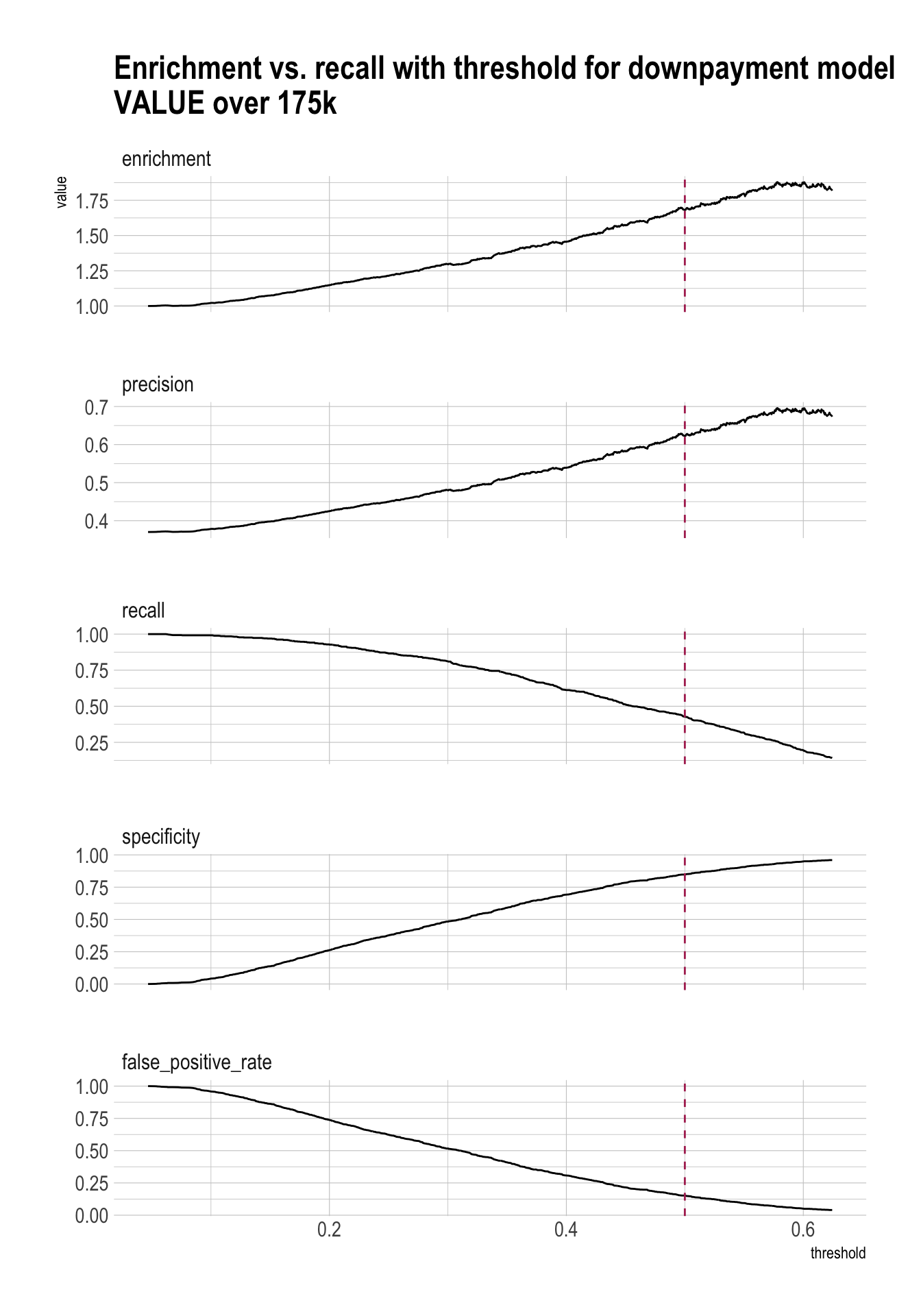
plt <- PRTPlot(df_cm_under_175k,
               ".fitted", "GT20DWN", 1,
               plotvars = c("enrichment", "precision", "recall", "specificity", "false_positive_rate"),
               thresholdrange = c(0, threshold_under_175k * 1.25),
               title = "Enrichment vs. recall with threshold for downpayment model\nVALUE under 175k")

plt +
  geom_vline(xintercept = threshold_under_175k,
             color="maroon",
             linetype = 2)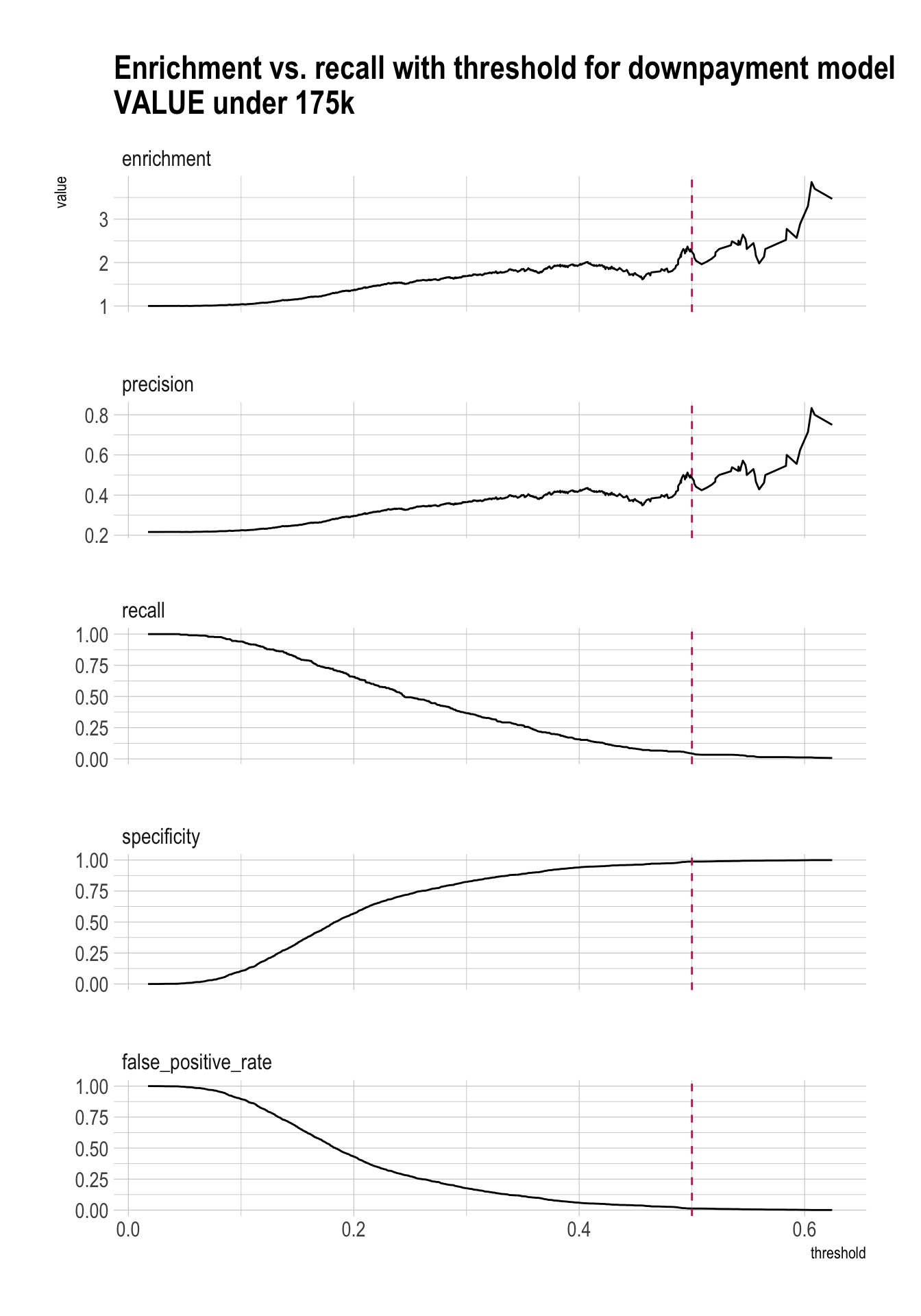
ROC
roc <- ROCPlot(df_cm_over_175k,
               xvar = '.fitted',
               truthVar = 'GT20DWN',
               truthTarget = 1,
               title = 'Classifier performance\nVALUE over 175k')

# ROC with vertical line
roc +
  geom_vline(xintercept = 1 - specificity_over_175k,
             color="maroon", linetype = 2)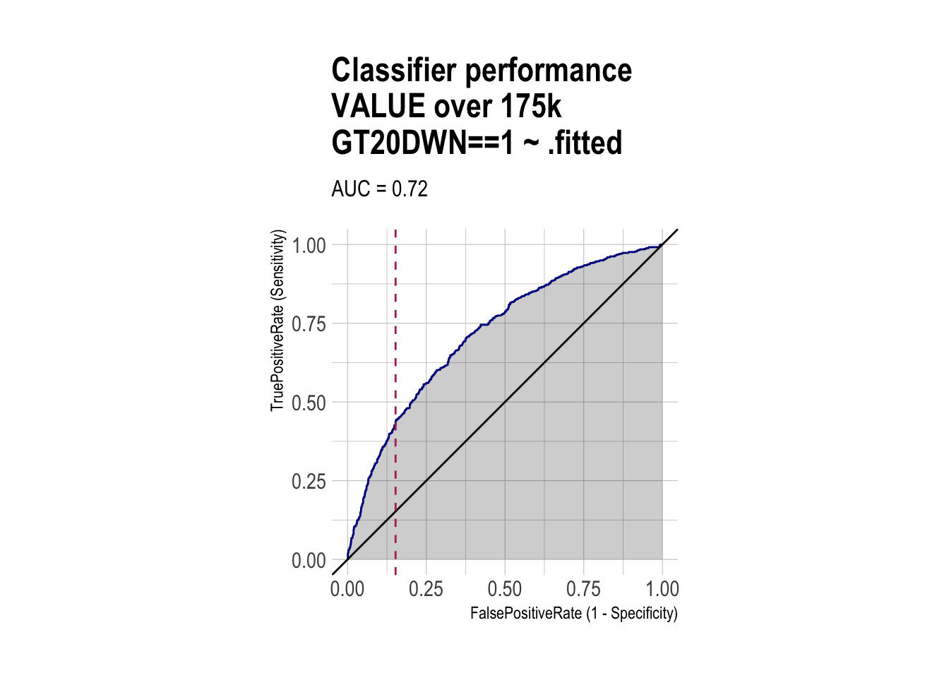
roc <- ROCPlot(df_cm_under_175k,
               xvar = '.fitted',
               truthVar = 'GT20DWN',
               truthTarget = 1,
               title = 'Classifier performance\nVALUE under 175k')

# ROC with vertical line
roc +
  geom_vline(xintercept = 1 - specificity_under_175k,
             color="maroon", linetype = 2)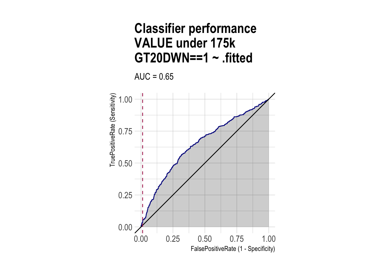
AUC
roc_obj_over_175k <- roc(df_cm_over_175k$GT20DWN, df_cm_over_175k$.fitted)
auc(roc_obj_over_175k)
Area under the curve: 0.7177roc_obj_under_175k <- roc(df_cm_under_175k$GT20DWN, df_cm_under_175k$.fitted)
auc(roc_obj_under_175k)Area under the curve: 0.6464Part 2 Task — Write a blog post (Quarto Document)
Write a blog post about Part 1 of Homework 2 - Beer Markets, and add it to your online blog.
Requirements (minimum):
Create a post using a Quarto Document (
.qmd) and ensure it appears on your Quarto website blog.Include:
- a short introduction (what the dataset is and what you’ll explore)
- descriptive statistics (at least 3 summary numbers)
- counting (e.g., top flavors)
- filtering (at least one meaningful filter)
- grouped summaries (at least one
group_by()+summarise()) - regression models in Homework 1
Optional but encouraged:
- at least one ggplot visualization
Deliverables:
- The blog post (in your website repo) renders successfully
- The post is accessible from your website’s blog listing page
- In your Brightspace submission (Part 1 QMD), include the URL to your published blog post