library(tidyverse)
library(janitor)
library(rpart)
library(rpart.plot)
library(broom)

library(DT)
library(rmarkdown)
library(hrbrthemes)
library(ggthemes)

theme_set(
  theme_ipsum()
)

scale_colour_discrete <- function(...) scale_color_colorblind(...)
scale_fill_discrete <- function(...) scale_fill_colorblind(...)Classwork 8
Decision Trees
Setup
Packages
library(tidyverse)
library(janitor)
library(rpart)
library(rpart.plot)
library(broom)
library(skimr)
Part 1. Regression Tree with MLB Batting Data
MLB Batting Data
mlb_data <- read_csv(
  "http://bcdanl.github.io/data/mlb_fg_batting_2022.csv"
) |>
  clean_names() |>
  mutate(across(bb_percent:k_percent, readr::parse_number))

mlb_data |>
  paged_table()
Variable Description
w_oba: weighted on-base average, a summary measure of offensive performancebb_percent: walk percentagek_percent: strikeout percentageiso: isolated poweravg: batting averageobp: on-base percentageslg: slugging percentagewar: wins above replacement
Explore the variables
mlb_data |>
  select(w_oba, bb_percent, k_percent, iso) |>
skimr::skim()| Name | select(mlb_data, w_oba, b… |
| Number of rows | 157 |
| Number of columns | 4 |
| _______________________ | |
| Column type frequency: | |
| numeric | 4 |
| ________________________ | |
| Group variables | None |
Variable type: numeric
| skim_variable | n_missing | complete_rate | mean | sd | p0 | p25 | p50 | p75 | p100 | hist |
|---|---|---|---|---|---|---|---|---|---|---|
| w_oba | 0 | 1 | 0.33 | 0.04 | 0.25 | 0.31 | 0.33 | 0.35 | 0.44 | ▃▇▇▃▁ |
| bb_percent | 0 | 1 | 8.80 | 2.97 | 3.50 | 6.50 | 8.60 | 11.00 | 20.30 | ▆▇▆▁▁ |
| k_percent | 0 | 1 | 20.47 | 5.89 | 8.10 | 16.10 | 19.90 | 24.80 | 36.10 | ▃▇▇▅▁ |
| iso | 0 | 1 | 0.17 | 0.06 | 0.05 | 0.12 | 0.17 | 0.20 | 0.35 | ▃▇▇▂▁ |
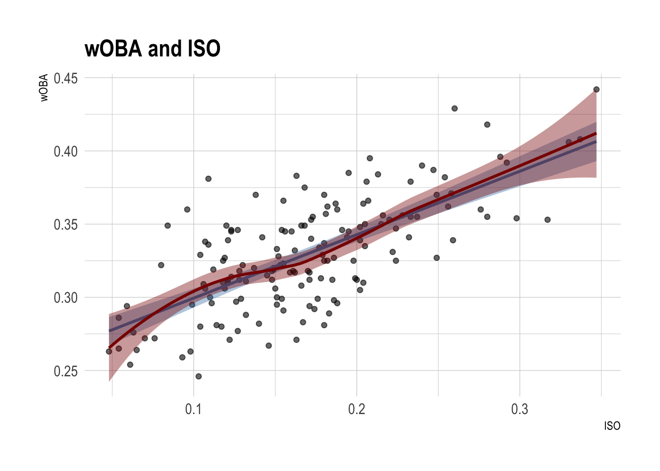
mlb_data |>
  ggplot(aes(x = iso, y = w_oba)) +
  geom_point(alpha = 0.6) +
  geom_smooth(method = lm,
              color = 'steelblue',
              fill = 'steelblue') +
  geom_smooth(color = 'red4',
              fill = 'red4') +
  labs(
    title = "wOBA and ISO",
    x = "ISO",
    y = "wOBA"
  )
Question 1. Fit an initial regression tree
Fit a simple regression tree using three predictors, bb_percent, k_percent, and iso.
- Do not specify any
controloptions inrpart().
# CODE HEREAnswer the following in complete sentences:
- Which variable appears at the first split?
- What does that suggest about the predictor’s importance in this tree?
- Choose one terminal node and explain what its predicted value means.
Question 2. Grow a larger tree
Now let the algorithm grow a much more flexible tree.
# CODE HEREAnswer the following:
- Compared with the first tree, is this tree more or less complex?
- Why might a very large tree be a problem for out-of-sample prediction?
- Looking at
plotcp(), what kind of tree are we usually trying to choose: the biggest tree, the smallest tree, or a tree that balances fit and complexity?
Question 3. Fine-tune tree growth before pruning
Before pruning, try a few different tree-growth settings. This is a simple form of hyperparameter tuning. The goal is to see how choices like minsplit and maxdepth affect the size of the tree and the cross-validated error.
reg_tuning_grid <- tribble(
  ~minsplit, ~maxdepth,
  20,        4,
  20,        6,
  40,        4,
  40,        6
)
# CODE HEREAnswer the following:
- Which combination of
minsplitandmaxdepthgives the smallest cross-validated error? - What does the
xerrorcolumn represent? Why do we often use it when choosing the pruning parameter? - Does a deeper tree always give the best
xerror? - Based on this table, which setting would you carry forward to pruning, and why?
Question 4. Prune the tuned tree
Fit a decision tree using the hyperparameter setting you prefer from Question 3.
Then prune the tuned tree.
# CODE HERECompare the tuned unpruned tree and the pruned tree.
- What became simpler after pruning?
- Why can a pruned tree sometimes predict better on new data even if it fits the training data less closely?
- Did your earlier hyperparameter choices seem to matter for the final pruned result?
Part 2. Classification Tree with MLB Batted-Ball Data
MLB batted-ball data
batted_ball_data <- read_csv(
  "http://bcdanl.github.io/data/mlb_batted_balls_2022.csv"
) |>
  mutate(is_hr = as.factor(events == "home_run")) |>
  filter(
    !is.na(launch_angle),
    !is.na(launch_speed),
    !is.na(is_hr)
  )

batted_ball_data |>
  paged_table()
batted_ball_data |>
count(is_hr) # A tibble: 2 × 2
is_hr n
<fct> <int>
1 FALSE 6702
2 TRUE 333Question 5. Visualize the classification problem
batted_ball_data |>
  ggplot(aes(x = launch_speed, y = launch_angle, color = is_hr)) +
  geom_point(alpha = 0.35) +
  labs(
    title = "Home Runs vs. Other Batted Balls",
    x = "Launch speed",
    y = "Launch angle",
    color = "Home run?"
  )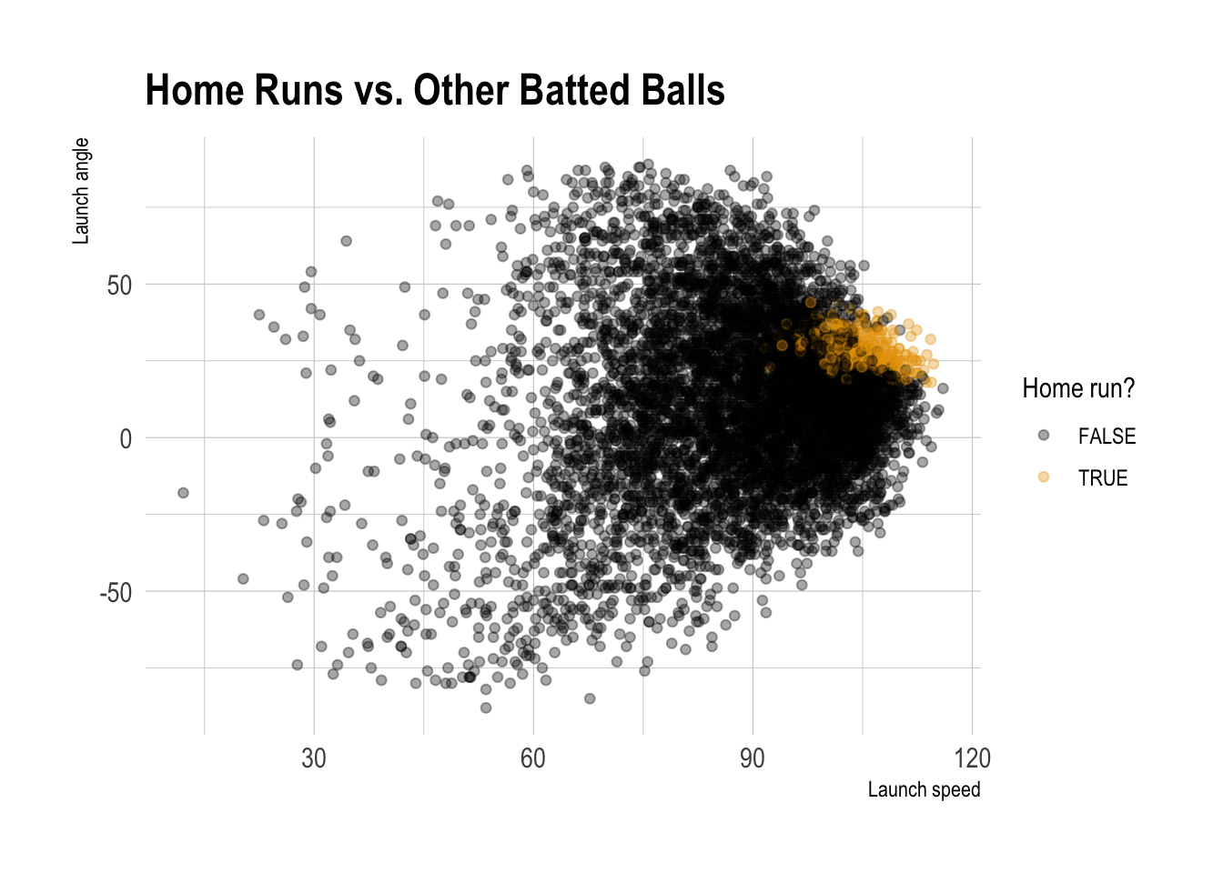
Based on the scatterplot, where do home runs seem more likely to happen? Describe the rough region using launch speed and launch angle.
Question 6. Train-test split
- Divide the
batted_ball_datadata.frame into training and test data.frames.- Use
dtrainanddtestfor training and test data.frames, respectively. - 70% of observations in the
batted_ball_dataare assigned todtrain; the rest is assigned todtest.
- Use
# CODE HEREQuestion 7. Fit a classification tree
Fit a simple classification tree using three predictors, launch_speed, launch_angle, and iso.
Do not specify any
controloptions inrpart().Which predictor appears to play a larger role near the top of the tree?
# CODE HEREQuestion 8. Tuning
Tune a classfication tree with the following hyperparameter settings:
cp = 0.0005minsplit = 30maxdepth = 5
Is the tuned tree more complex?
# CODE HEREQuestion 9. Classification
Build two classifiers using the original classification tree and tuned classification trees.
Compare the original classification tree and the tuned classification tree.
# CODE HEREDiscussion
Welcome to our Classwork 8 Discussion Board! 👋
This space is designed for you to engage with your classmates about the material covered in Classwork 8.
Whether you are looking to delve deeper into the content, share insights, or have questions about the content, this is the perfect place for you.
If you have any specific questions for Byeong-Hak (@bcdanl) regarding the Classwork 8 materials or need clarification on any points, don’t hesitate to ask here.
All comments will be stored here.
Let’s collaborate and learn from each other!