Lecture 5
Data Wrangling with tidyr, forcats, and stringr
March 2, 2026
Tidy Data
What Are Tidy Data?
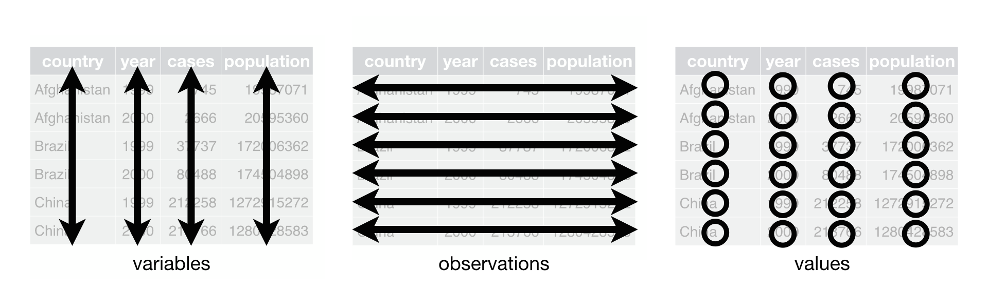
There are three rules which make a dataset tidy:
- Each variable must have its own column.
- Each observation must have its own row.
- Each value must have its own cell.
Tidy data
- We can represent the same underlying data in multiple ways.
🔄 Pivoting
Pivoting
- The first step is always to figure out what form of the variables and observations we need.
- The second step is to resolve one of two common problems:
- One variable might be spread across multiple columns.
- One observation might be scattered across multiple rows.
- To fix these problems, we may need the two most important functions in the
tidyrpackage:pivot_longer()andpivot_wider().
Longer
Some of the column names are not names of variables, but values of a variable.
We use
pivot_longer()when a variable might be spread across multiple columns.
Longer
To tidy a dataset like
table4a, we need to pivot the offending columns into a new pair of variables.To use
pivot_longer(), we need to the following three parameters:- The set of columns (
cols) whose names are values, not variables. - The name of the variable to move the column names to (
names_to). - The name of the variable to move the column values to (
values_to).
- The set of columns (
Longer
Wider
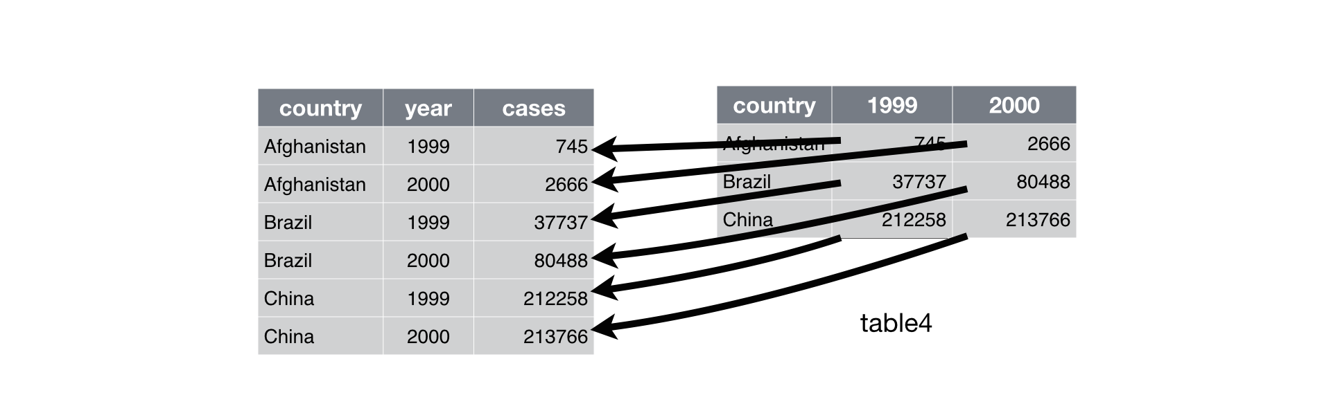
One observation might be scattered across multiple rows.
We use
pivot_wider()when an observation is scattered across multiple rows.
Wider
- To use
pivot_wider(), we need two parameters:- The column to take variable names from.
- The column to take values from.
- We can add the optimal parameter,
names_prefix, for the prefix of column names.
Wider

✂️ Separating and Uniting
Separating a Column with separate()
table3has one column (rate) that contains two variables (casesandpopulation).separate()takes the name of the column to separate, and the names of the columns to separate into.
Separating a Column with separate()
- If we want to use a specific chracter to seprate a column, we can pass the character to the
sepparameter.
Separating a Column with separate()
- By default,
separate()leaves the type of the column as is.
Separating a Column with separate()
separate()will interpret the integers as positions to split at.We can also pass a vector of integers to
sep.separate()will interpret the integer as positions to split at.
Uniting Columns into a Single Column with unite()
unite()combines multiple columns into a single column.The default will place an underscore (
_) between the values from different columns.
🔗 Relational Data
Relational data
It’s rare that a data analysis involves only a single data frame.
Collectively, multiple data frames are called relational data.
To work with relational data, we need verbs that work with pairs of data frames.
join methods add new variables to one data frame from matching observations in another data frame.
nycflights13
nycflights13contains four data frames that are related to the data frame,flights, that we used in data transformation.
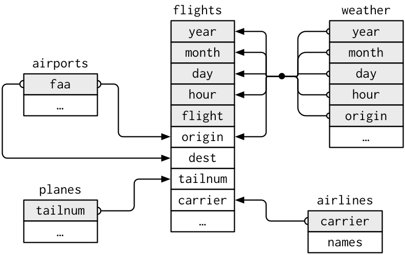
nycflights13
flightsconnects to …planesvia a single variable,tailnum.airlinesthrough thecarriervariable.airportsin two ways: via theoriginanddestvariables.weatherviaorigin(the location), andyear,month,dayandhour(the time).
Relations in nycflights13
Key Variables
A key variable (or a set of key variables) is a variable (or a set of variables) that uniquely identifies an observation.
So, a key variable (or a set of key variables) is used to connect relational data.frames.
The name of a key variable can be different across relational data.frames.
Relational Data
- A join allows us to combine two data frames via key variables.
- It first matches observations by their keys, then copies across variables from one data.frame to the other.
| Tidyverse | SQL | Description |
|---|---|---|
| left | left outer | Keep all the observations from the left |
| right | right outer | Keep all the observations from the right |
| full | full outer | Keep all the observations from both left and right |
| inner | inner | Keep only the observations whose key values exist in both |
Joins
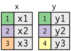
- The colored column represents the “key” variable.
- The grey column represents the “value” column.
Joining Tables with inner_join()
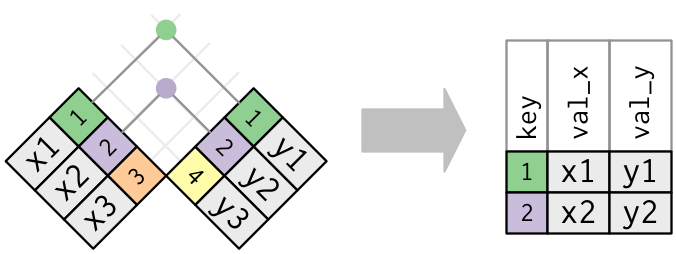
- An inner join matches pairs of observations whenever their keys are equal:
Joining Tables with left_join()
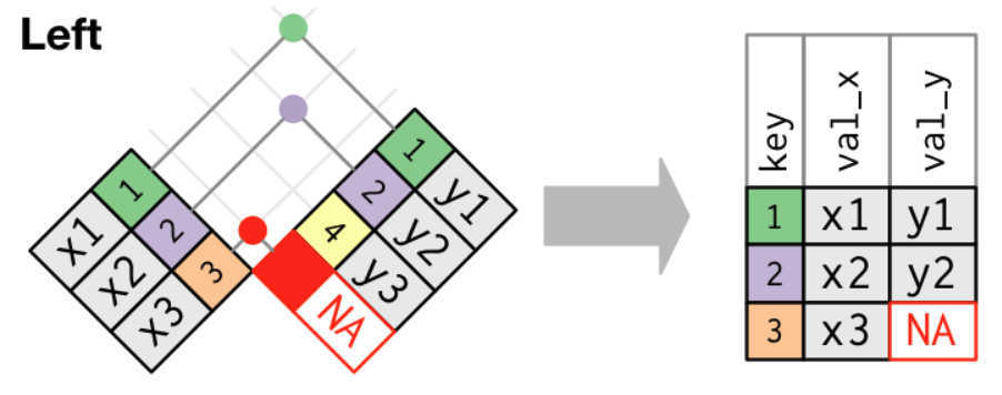
- A left join keeps all rows from
xand adds matching information fromy. - Among the different join types,
left_join()is the most commonly used join.- It does not lose information from your main data.frame (
x) and simply attaches extra information (y) when it exists.
- It does not lose information from your main data.frame (
Joining Tables with right_join()
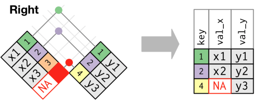
- A right join keeps all observations in
y.
Joining Tables with full_join()
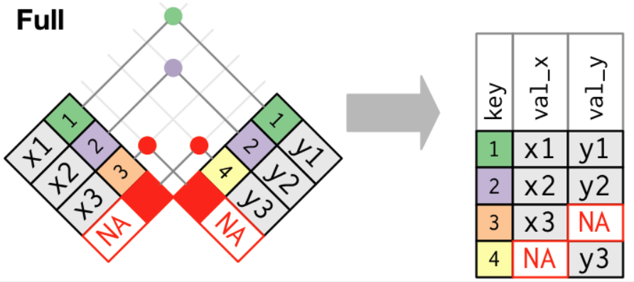
- A full join keeps all observations in
xandy.
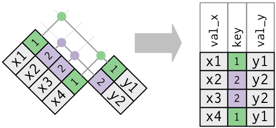
Duplicate Keys
- Relations between data.frames could be …
- One-to-one;
- One-to-many (e.g.,
airlinesandairports); - Many-to-one;
- Many-to-many (e.g.,
flightsandairplanes).
- One-to-many relation is such that one data.frame has duplicate keys
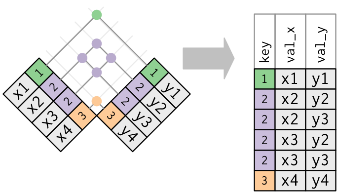
- Many-to-many relation is such that both data.frames have duplicate keys.
- In practice, it is recommended to avoid joining data.frames with many-to-many relation.
Duplicate Keys: One-to-many Join
Duplicate Keys: Many-to-many Join
Joins: Defining the Key Columns
by = "a": uses only variablea.by = c("a" = "b"): match variableain data framexto variablebin data framey.
🧩 Data Assembly
🧩 Data Assembly
Row-bind (stack rows): rbind() vs. bind_rows()
rbind()(base R) requires the same columns in the same order (and compatible types). If names/order don’t match, it typically errors.bind_rows()(dplyr) matches columns by name, and will fill missing columns withNAwhen the inputs have different sets of columns.- Tip: use
bind_rows()when combining files that may have slightly different columns (common in real data).
Column-bind (add columns side-by-side): cbind() vs. bind_cols()
cbind()(base R) binds by row position and can silently coerce to a matrix (e.g., mixing numbers + strings) and may recycle shorter vectors in some cases.bind_cols()(dplyr) also binds by row position, but is stricter about row counts and returns a tibble with safer name handling.- Tip: column-binding is best when the rows are already in the same order; if you need to match by a key (e.g.,
id), use a join (left_join,inner_join) instead.
Data Assembly: rbind() vs. bind_rows()
rbind()typically fails when the two data.frames have different column names.bind_rows()can still work because it matches columns by name and fills the rest withNA.
Data Assembly: cbind() vs. bind_cols()
- Both
cbind()andbind_cols()require compatible row counts; otherwise it errors.
Factors
Creating Factors
- In
R, factors are categorical variables, variables that have a fixed and known set of possible values.
Creating Factors with factor()
- We can fix both of these problems with
factor(). - To create a factor, we must start by creating a list of the valid
levels. - Any values not in the set will be silently converted to
NA. - If we omit the
levels, they’ll be taken from the data in alphabetical order:
Creating Factors with factor()
Sometimes we’d prefer that the order of the levels match the order of the first appearance in the data.
We can do that when creating the factor by setting levels to
unique().If we ever need to access the set of valid levels directly, we can do so with
levels().
Creating Factors with factor(): labels Option
- The
labelsoption infactor()allows us to assign custom display names to the levels. - The
labelsmust be in the same order as thelevels.
- Without
labels, factor levels display as-is; withlabels, we control how they appear in outputs and plots.
Data: General Social Survey
We’re going to focus on the data frame,
forcats::gss_cat.which is a sample of data from the General Social Survey.When factors are stored in a data frame, we can see them with
count().
Modifying Factor Order
It’s often useful to change the order of the factor levels in a visualization.
Imagine we want to explore the average number of hours spent watching TV per day across
relig.
Modifying Factor Order with fct_reorder(f, x, fun)
We can reorder the levels using
fct_reorder(f, x, fun), which can take three arguments.f: the factor whose levels we want to modify.x: a numeric vector that we want to use to reorder the levels.Optionally,
fun: a function that’s used if there are multiple values ofxfor each value off. The default value is median.
Modifying Factor Order with fct_reorder2(f, x, y) 🔀
by_age <- gss_cat |>
  filter(!is.na(age)) |>
  count(age, marital) |>
  group_by(age) |>
  mutate(prop = n / sum(n))

# Default legend order (alphabetical)
ggplot(by_age, aes(x = age, y = prop, color = marital)) +
  geom_line(linewidth = 1) +
  scale_color_brewer(palette = "Set1")

# Legend order follows the line endings at the largest age
ggplot(by_age, aes(x = age, y = prop,
                   color = fct_reorder2(marital, age, prop))) +
  geom_line(linewidth = 1) +
  scale_color_brewer(palette = "Set1") +
  labs(color = "marital")
Modifying Factor Order with fct_reorder2(f, x, y) 🔀
fct_reorder2(f, x, y) (from forcats) is useful when you have multiple lines (one per factor level) and you want the legend order to follow the right-end (or left-end) of the lines.
f: the factor you want to reorder (e.g.,marital)x: the horizontal variable (e.g.,age)y: the numeric outcome used to rank levels (e.g.,prop)- It orders factor levels by the
yvalue at the largestx(i.e., near the right edge of the plot).- This makes the legend easier to read because the legend order matches where lines end up on the right.
Modifying Factor Order with fct_relevel(x, ref = ...)
- We can use
fct_relevel()to set the first level (reference level). fct_relevel(x, ref = ...)takes at least the two arguments:x: factor variableref: reference level or first level
🔤 Strings
Combining Strings with str_c()
To count the length of string, use
str_length().To combine two or more strings, use
str_c():To control how strings are separated, add the
sep.To collapse a vector of strings into a single string, add the
collapse.
Subsetting Strings str_sub()
We can extract parts of a string using
str_sub():str_sub()takesstartandendarguments which give the position of the substring.
Matching a Pattern of Strings: str_detect() and str_replace_all()
- To determine if a character vector matches a pattern, use
str_detect(). str_replace()andstr_replace_all()allow us to replace matches with new strings.str_replace_all()can perform multiple replacements by supplying a named vector.
Splitting Strings with str_split()
- Use
str_split()to split a string up into pieces.