Lecture 3
Data Transformation with dplyr
February 9, 2026
Reading a Data Table as a data.frame
📍 Absolute Pathnames
- An absolute pathname tells the computer the full, exact location of a file, starting from the top-level folder of the computer.
- Because it starts from the top, it does not depend on your current working directory.
- In R, you can check your working directory (the folder R is currently “looking in” by default) by running:
📎 Relative Pathnames
- A relative pathname gives a file location relative to the working directory.
- In many web-related projects (and collaborative projects), relative paths are almost necessary.
- Suppose your working directory is
and your file is stored at:
🔎 Getting to Know a data.frame
Basic structure + a single column
Size of the data.frame
Column names
- The
$operator extracts a single column from adata.frameas a vector (e.g.,custdata$age).
nrow()/ncol()returns the number of rows/columns.
colnames()returns a character vector of column names.
Quick Summary with skimr::skim()
skimr::skim()quickly summarizes types, missing values, and key descriptive stats, and it works well with pipes and grouped data (e.g.,custdata |> dplyr::group_by(state_or_res) |> skimr::skim()).
Tidy data.frame
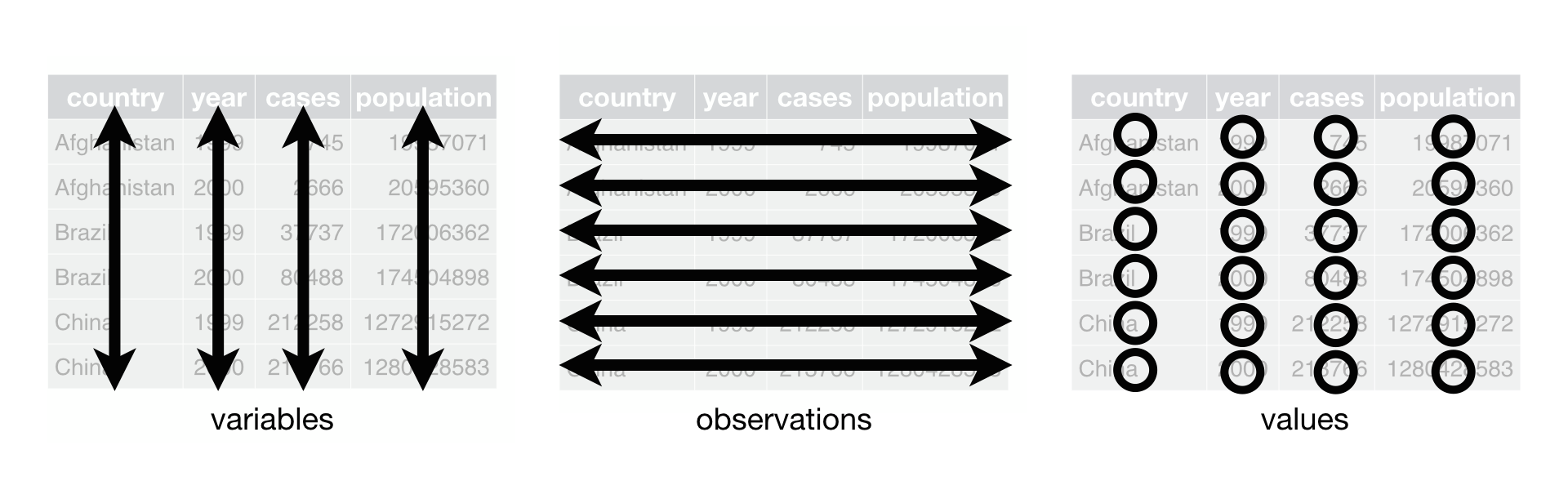
- Rows represent individual units (observations) where data is collected.
- Columns represent variables (attributes) measured for each observation.
- Tidy data is easier to read, analyze, and share.
- A
data.frameis tidy when it follows three rules:- Each variable is a column.
- Each observation is a row.
- Each value is a cell.
- Each variable is a column.
Data Transformation
Data Transformation with dplyr
dplyris a core tidyverse package for data manipulation — tasks like filtering, sorting, selecting, renaming, and many more. Commondplyrfunctions with data.frameDF:
filter(DF, LOGICAL_COND)
arrange(DF, VARIABLES)
distinct(DF, VARIABLES)
select(DF, VARIABLES)
relocate(DF, VARIABLES)
rename(DF, NEW_NAME = CURRENT_NAME)
mutate(DF, NEW_NAME = CURRENT_NAME)
group_by(DF, VARIABLES)
summarize(DF, NEW_NAME = CURRENT_NAME)
slice_*(DF, VARIABLE, n = ..)
dplyrfunctions take a data.frame as the first argument, and return a data.frame as output.
Making dplyr Code Flow with the Pipe Operator
- The pipe operator (
|>or%>%) makes code easier to read by connecting steps in order.
- How it works:
f(x, y)is the same asx |> f(y).
- Example with a data frame
DF:filter(DF, logical_condition)
- is the same as
DF |> filter(logical_condition)
- You can read the pipe as “then”:
- Example: Take the data, then filter it
Data Transformation with the Pipe
DF |> filter(LOGICAL_CONDITIONS)
DF |> arrange(VARIABLES)
DF |> distinct(VARIABLES)
DF |> select(VARIABLES)
DF |> relocate(VARIABLES)
DF |> rename(NEW_NAME = CURRENT_NAME)
DF |> mutate(NEW_NAME = CURRENT_NAME)
DF |> group_by(VARIABLES)
DF |> summarize(NEW_NAME = CURRENT_NAME)
DF |> slice_*(VARIABLE, n = ..)This allows you to chain together multiple steps naturally:
Start with data, then filter, then arrange
DF |> filter(...) |> arrange(...)
Using the Pipe in RStudio
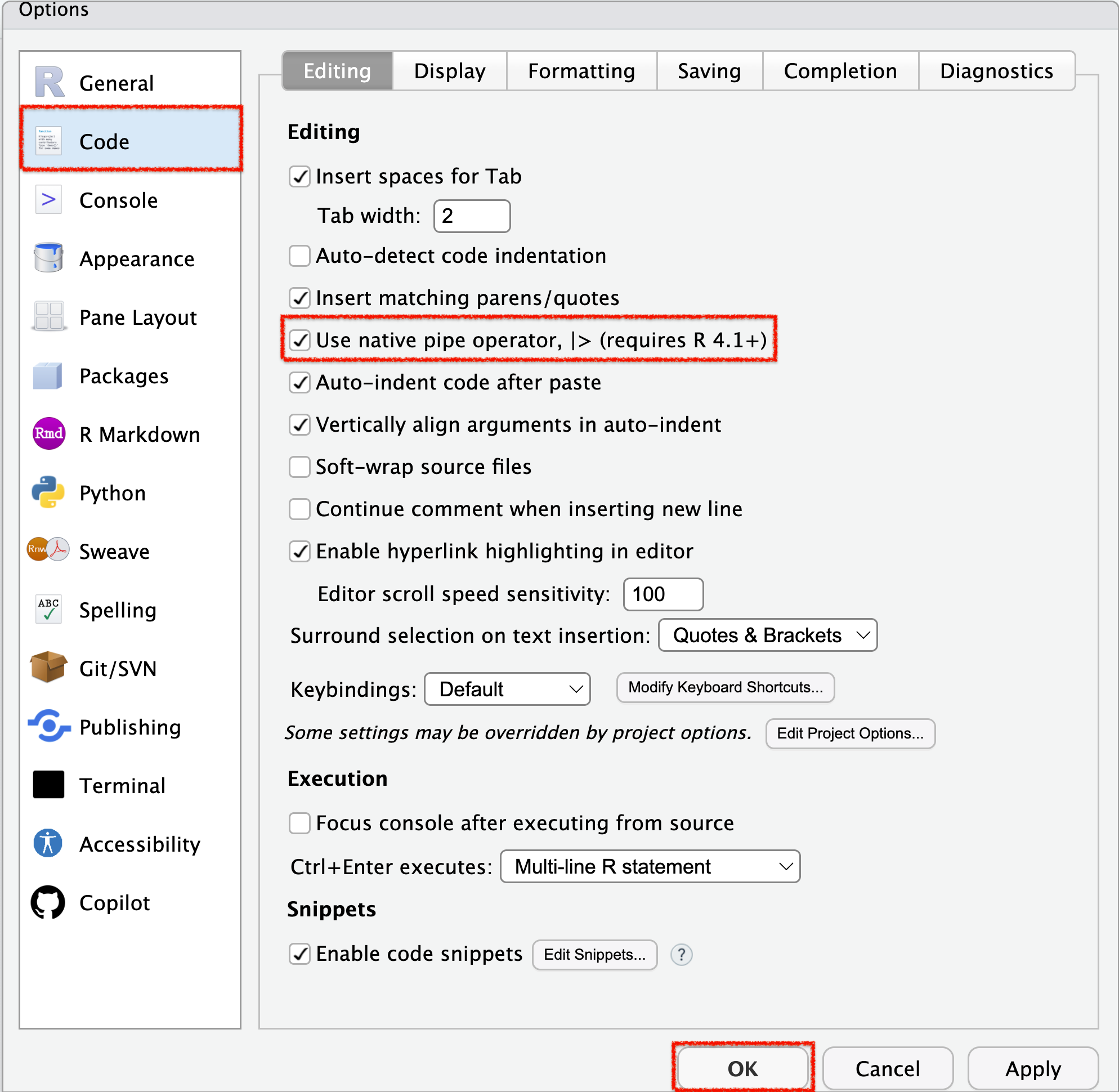
- To enable the native pipe operator (
|>) in RStudio:- Go to Tools > Global Options > Code (side menu).
- Under Pipe operator, choose Use native pipe operator (
|>).
- Go to Tools > Global Options > Code (side menu).
- Keyboard shortcut for inserting a pipe:
- Windows: Ctrl + Shift + M
- Mac: Cmd + Shift + M
- Windows: Ctrl + Shift + M
Filter observations with filter()
Filter Observations with filter()
install.packages("nycflights13")  # Install once
library(nycflights13)
library(tidyverse)

flights <- nycflights13::flights

flights$month == 1  # A logical test returns TRUE or FALSE
class(flights$month == 12) filter()keeps only the observations that meet one or more logical conditions.- A logical condition evaluates to
TRUE(keep the observation) orFALSE(drop the observation).
- A logical condition evaluates to
Logical Conditions with Equality and Inequality
- Here, both
V1andV2are variables, and the comparisons are applied element-wise (vectorized).
- For logical conditions using inequalities, we focus on cases where
V1andV2areintegerornumeric.
Logical Conditions - Example 1
Logical Operators — AND, OR, NOT
- Here, both
xandyarelogicalconditions/variables.
- What logical operations (
&,|,!) do is combining logical variables/conditions, which returns alogicalvariable when executed.
Logical Operations
xandyare logical conditions.- If
xisTRUE, it highlights the left circle.
- If
yisTRUE, it highlights the right circle.
- If
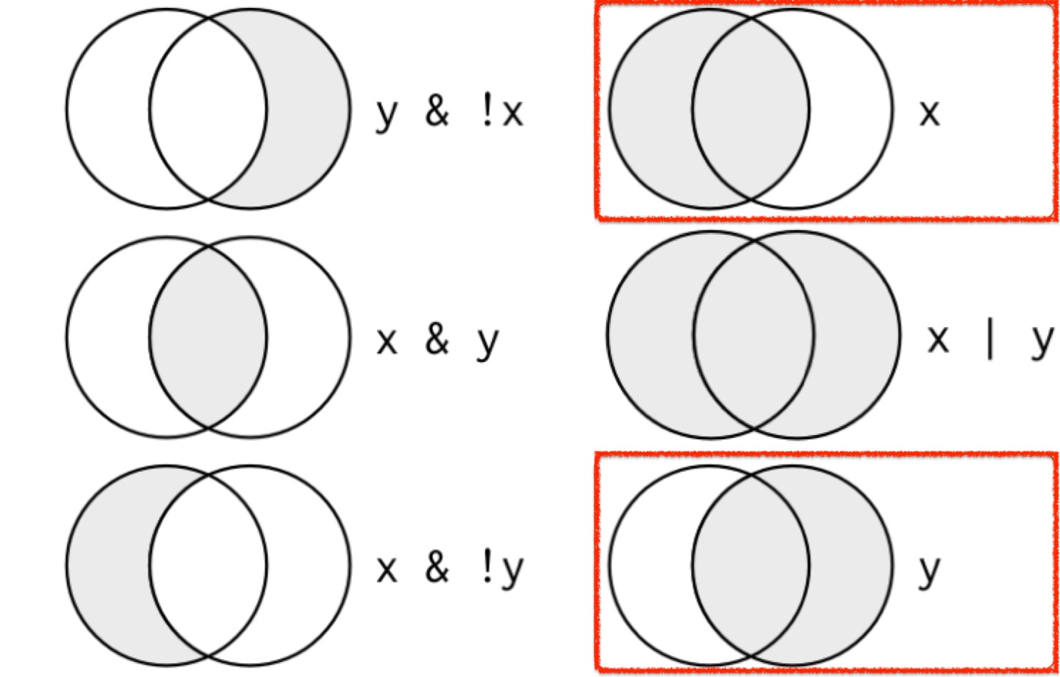
- The shaded regions show which parts each logical operator selects.
Logical Conditions - Example 2
- In
filter(), separating conditions with a comma is equivalent to combining them with the&operator.
Logical Conditions - Example 3
Logical Conditions - Example 4
Missing Values (NA)
NA(not available) represents a missing or unknown value in R.
- In most calculations, if one value is unknown, the result will also be unknown (
NA).
Comparing Missing Values
- Suppose
v1is Mary’s age (unknown) andv2is John’s age (unknown). - Can we say they are the same age?
- Since both values are missing, R cannot know — so the result is also
NA.
Checking for Missing Values with is.na()
- Use
is.na()to test whether a value is missing (NA).
- In
filter(), you can:- Use
is.na()to keep observations with missing values. - Use
!is.na()to remove observations with missing values.
- Use
Arrange Observations with arrange()
Arrange Observations with arrange()
arrange()sorts out observations.- When you provide multiple variables,
arrange()sorts by the first variable, and then uses the next variable(s) to break ties.
Descending Order with desc()
- Use
desc(VARIABLE)to sort in descending order.- For numeric variables, you can also use a leading minus sign.
Arrange Observations with arrange() - Example
- If we provide more than one variable name, each additional variable will be used to break ties in the values of preceding variables.
Find All Unique Observations with distinct()
Find All Unique Observations with distinct()
distinct()removes duplicate observations.- By default, it checks all variables to find unique observations.
Find All Unique Combinations of Selected Variables
- You can pass one or more variables to
distinct().- This returns unique combinations of just those variables (while ignoring the rest).
Select Variables with select()
Select Variables with select()
It’s not uncommon to get datasets with hundreds or thousands of variables.
select()allows us to narrow in on the variables we’re actually interested in.We can select variables by their names.
Remove Variables with select()
- With
select(-VARIABLES), we can remove variables.
Helper Functions with select()
- There are a number of helper functions we can use within
select():starts_with("abc"): matches names that begin with “abc”.ends_with("xyz"): matches names that end with “xyz”.contains("ijk"): matches names that contain “ijk”.num_range("x", 1:3): matches x1, x2 and x3.
Rename Variables with rename()
Rename Variables with rename()
rename()can be used to rename variables:DF |> rename(NEW_NAME = CURRENT_NAME)
Relocate Variables with relocate()
Relocate Variables with relocate()
- We can use
relocate()to move variables around.
relocate() with .before or .after
- We can also use
relocate()to move variables around.- We can specify
.beforeand.afterarguments to choose where to put variables:
- We can specify
Add New Variables with mutate()
Add New Variables with mutate()
- We can use the
mutate()to add variables to the data.frame:
mutate() with .before or .after
- We can use the
.beforeor.afterargument to add the variables to the position of a column - The
.is a sign that.beforeis an argument to the function, not the name of variable. - In both
.beforeand.after, we can use the variable name instead of a position number.
mutate() with Offsets and Cumulative Functions
Offsets let you reference the previous or next value (useful for changes over time). Cumulative functions build running totals (or running mins/maxes).
mutate() with Ranking Functions
Ranking helpers are great for creating order, percentiles, or within-group standings.
rank_me <- data.frame(x = c(10, 5, 1, 5, 5, NA))

rank_me |>
  mutate(
    id = row_number(),             # row id (1, 2, 3, ...)
    x_row_number = row_number(x),  # tie-breaking rank (arbitrary but stable)
    x_min_rank   = min_rank(x),    # ranks with gaps when ties occur
    x_dense_rank = dense_rank(x),  # ranks without gaps when ties occur
    x_percent    = percent_rank(x),# 0 to 1 (excluding 1 unless max)
    x_cume       = cume_dist(x)    # 0 to 1 (including 1 for max)
  )
mutate() with if_else() or ifelse()
Use conditional functions to create a new variable based on a rule.
if_else()
- Strict: both outputs must be the same type (both logical, both numeric, both character, etc.).
if_else() vs. ifelse()
- Use
if_else()when you want type safety (both outcomes must match). - Use
ifelse()only when you intentionally accept coercion
mutate() with case_when()
- Use
case_when()when you have 3+ conditions (an “if-else” chain). - Order matters: the first matching condition is used.
- Recommend including a default case:
TRUE ~ ...- Without
TRUE ~ ..., any observation that doesn’t match your listed conditions becomesNA.
- Without
Grouped Summaries with summarize()
summarize() in one sentence
summarize()reduces rows by computing summary statistics.- Without
group_by(), you get one row for the entire dataset. - With
group_by(...), you get one row per group.
Mental model
group_by() splits → summarize() reduces → output combines
What Happens When We Group Then Summarize?
Split-Apply-Combine
Key idea
group_by(cat2)splits the data into groups (one group percat2value).summarize(...)collapses each group down to one row (one row per group).
Example: Destination-level Summaries
Goal: For each destination (dest), compute
(1) number of flights, (2) average distance, (3) average arrival delay.
Missing Values: Why na.rm = TRUE Matters
If you don’t remove missing values, many summaries become NA.
If Missing Means “cancelled”
A common approach is to create a dataset of not-cancelled flights first.
Counts: always include a size check
When you compute an average, include a count so you don’t trust tiny groups.
Useful Summary Functions: Location (Center)
Mean: mean(x)
- Average value (adds values and divides by count)
- Use
na.rm = TRUEif there are missing values
Useful Summary Functions: Spread (Variation)
Standard deviation: sd(x)
- Typical distance from the mean
- Bigger
sd→ more variability
Minimum / maximum: min(x), max(x)
- Smallest and largest values in a group
Quantiles: quantile(x, p)
- Value at percentile
p(e.g., 25th percentile)
Range: range(x)
- Returns both min and max together
First / last: first(x), last(x)
- First and last values in the current row order
- If you need a specific definition of “first”, sort first!
Nth: nth(x, n)
- The n-th value in the current order
Conditional Subsetting Inside a Summary
Example: arr_delay[arr_delay > 0]
- Inside a summary, you can “filter” a single column using brackets
[] arr_delay[arr_delay > 0]means:
keep only the values ofarr_delaythat are greater than 0
Why do this?
avg_delaycan be pulled down by early flights (negative delays)avg_pos_delayanswers: “When flights are late, how late are they on average?”
When do the first and last flights leave each day?
Option A: min / max (robust)
Option B: first / last (order-dependent)
Counting helpers
n()counts rows in each groupsum(!is.na(x))counts non-missing valuesn_distinct(x)counts distinct valuescount(x)is a shortcut forgroup_by(x) |> summarize(n = n())
Counts inside ggplot: histogram bins
A histogram is basically “count by bins”.
Logical Summaries: Counts + Proportions
sum(condition)counts how many areTRUE
Grouping by Multiple Variables: “Peeling” Groups
Each summarize() removes one layer of grouping by default.
Ungrouping
Use ungroup() when you want to stop doing per-group operations.
Grouped mutate() and filter()
Grouped mutate() and filter()
Grouping is most common with summarize(), but it can also help with:
- filtering within groups (e.g., “worst flights per day”)
- creating per-group metrics (e.g., “share of delay within a destination”)
Example 1: “worst” within each group
Goal: find (about) the 10 worst arrival delays within each day.
Example 2: groups above a threshold
Goal: keep only destinations with lots of flights.
Example 3: per-group metrics with mutate()
Goal: within each destination-day group, compute each flight’s share of total delay.
Grouped slice_*()
The slice_*() Functions
There are five handy functions that allow you to extract specific rows within each group:
grouped_df |> slice_head(n = 1)takes the first row.grouped_df |> slice_tail(n = 1)takes the last row.grouped_df |> slice_min(x, n = 1)takes the row with the smallest value of columnx.grouped_df |> slice_max(x, n = 1)takes the row with the largest value of columnx.grouped_df |> slice_sample(n = 1)takes one random row.- You can vary
nto select more than one row. - Instead of
n =, you can useprop = 0.1to select (e.g.) 10% of the rows in each group.
slice_head()
slice_head(n = 2)returns the first 2 rows for each destination group.- Useful for quickly previewing the earliest recorded observations per group.
slice_tail()
slice_tail(n = 2)returns the last 2 rows for each destination group.- Useful for inspecting the most recently recorded observations per group.
slice_min()
slice_min(arr_delay, n = 1)returns the flight with the smallest arrival delay for each destination.- Ties are kept by default.
- Use
with_ties = FALSEto return exactlynrows.
- Use
slice_max()
slice_max(arr_delay, n = 1)returns the flight with the longest arrival delay for each destination.- Ties are kept by default.
- Use
with_ties = FALSEto return exactlynrows.
- Use
- Great for identifying worst-case observations within each group.
slice_sample()
slice_sample(n = 1)draws one random flight from each destination group.- Use
prop = 0.1to randomly sample 10% of rows per group instead of a fixedn. - Results will differ each run — set
set.seed()beforehand for reproducibility.